Readout and fridge wiring

Measure three resonators through a common bus and a fridge readout line, then sample the VNA trace at two integration times. Frequencies are in GHz, times in ns, temperatures in mK, and decay rates in 1/ns. Run the cells in order.

Couple the resonators to a bus

The resonators are at 6.4, 6.5, and 6.6 GHz, each with its own internal loss. All three exchange photons with a 6.5 GHz bus, which has a 1 GHz external linewidth and connects to the measurement line. The resonators’ nominal loaded linewidths are 11–18 MHz.

import numpy as np
from scipy.signal import butter
from quchip import Capacitive, Chip, IQReceiver, PortNetwork, Resonator, RWA, VNA, qnp

mode_frequencies = np.array([6.4, 6.5, 6.6])
internal_q = np.array([1800, 3200, 2400])
external_q = np.array([450, 750, 550])

bus = Resonator(freq=6.5, levels=3, internal_quality_factor=100_000, label="bus")
resonators = [Resonator(freq=f, levels=3, internal_quality_factor=qi, label=f"r{i+1}")
              for i, (f, qi) in enumerate(zip(mode_frequencies, internal_q))]

bus_qe = 6.5
bus_external_rate = 2 * np.pi * bus.freq / bus_qe
bus_total_rate = bus_external_rate + 2 * np.pi * bus.freq / bus.internal_quality_factor
external_rates = 2 * np.pi * mode_frequencies / external_q
coupling_strengths = np.sqrt(external_rates * (
    (bus_total_rate / 2)**2 + (2 * np.pi * (mode_frequencies - bus.freq))**2
) / bus_external_rate) / (2 * np.pi)

couplings = [Capacitive(bus, r, g=g, label=f"bus_r{i+1}")
             for i, (r, g) in enumerate(zip(resonators, coupling_strengths))]

internal_quality_factor sets each resonator’s intrinsic decay. We set the couplings from a nominal external Q, with the bus susceptibility at each bare resonator frequency:

\[\kappa_{e,r} = \frac{(2\pi g_r)^2\,\kappa_{e,b}} {(\kappa_b/2)^2 + [2\pi(f_r-f_b)]^2}, \qquad Q_{e,r}=\frac{2\pi f_r}{\kappa_{e,r}}.\]

The simulation includes all three couplings, so the resonances shift and their linewidths change through the shared bus. RWA keeps the photon-exchange terms. The parameters are representative.

Put the chip in the fridge

A mixing-chamber circulator sends port 1 to the bus on port 2 and the reflection to port 3. The input attenuation is distributed across 4 K, the cold plate, and the mixing chamber. Two output isolators precede the 4 K HEMT. Both lines contain a 4–8 GHz bandpass filter.

filter_b, filter_a = butter(4, [4.0, 8.0], btype="bandpass", analog=True)


def passband(frequency):
    return qnp.polyval(filter_b, 1j * frequency) / qnp.polyval(filter_a, 1j * frequency)


fridge = PortNetwork(label="thermal_fridge")
port = fridge.port("bus_coupler", target=bus, external_quality_factor=bus_qe)
input_filter = fridge.filter("input_4_8GHz", transfer=passband)

n_4k, n_cp, n_mxc = 12.329033161427, 0.046220887106121, 1.6829628323748e-07
att_4k = fridge.attenuator("att_4K", loss_db=20, thermal_occupation=n_4k)
att_cp = fridge.attenuator("att_CP", loss_db=20, thermal_occupation=n_cp)
att_mxc = fridge.attenuator("att_MXC", loss_db=20, thermal_occupation=n_mxc)

circ = fridge.circulator("circ")
iso_1 = fridge.isolator("iso_1", thermal_occupation=n_mxc)
iso_2 = fridge.isolator("iso_2", thermal_occupation=n_mxc)
iso_loss = fridge.attenuator("iso_insertion", loss_db=1, thermal_occupation=n_mxc)
output_filter = fridge.filter("output_4_8GHz", transfer=passband,
                              thermal_occupation=n_mxc)

coax = fridge.attenuator("output_coax", loss_db=2, thermal_occupation=n_4k)
hemt = fridge.amplifier("HEMT_4K", gain_db=40, added_noise=8.0140842782029)
room_amp = fridge.amplifier("amp_RT", gain_db=20, added_noise=925.22946424527)

loss_db is the power loss in dB. thermal_occupation is the mean thermal population of a passive load in quanta. The values above correspond to 4 K, 100 mK, and 20 mK at 6.5 GHz and stay fixed in this sweep. The isolators use the coldest load, and iso_loss represents their combined insertion loss. The ideal circulator adds no noise of its own.

Amplifier added_noise is input-referred symmetrized noise in quanta. At 6.5 GHz, the HEMT value corresponds to a 2.5 K equivalent noise temperature, and the room amplifier value to a 3 dB noise figure referenced to 290 K. These values are fixed model inputs, independent of the amplifiers’ physical stages.

The filters have half-power edges at 4 and 8 GHz. The output filter’s thermal_occupation declares a matched absorptive load. The input filter sees a vacuum source, with thermal attenuators downstream. The resonators’ intrinsic loss baths are vacuum too.

Connect the input chain to circulator port 1, the bus to port 2, and the receiver chain to port 3. Name the external network ports drive for the source and readout for the receiver. Each port defines a reference plane, where the port’s incoming and outgoing fields are specified.

fridge.link(input_filter, att_4k, att_cp, att_mxc, circ.port(1))
fridge.link(circ.port(2), port)
fridge.link(circ.port(3), iso_1, iso_loss, iso_2, output_filter, coax, hemt, room_amp)
drive = fridge.expose("drive", at=input_filter.port(1))
readout = fridge.expose("readout", at=room_amp.port(2))
readout_chip = Chip([bus, *resonators], couplings, port_network=fridge,
                    approximation=RWA(), frame="rotating")

Draw the fridge wiring

import shutil
import matplotlib.pyplot as plt
from matplotlib.patches import Arc, Circle, FancyArrowPatch, Polygon, Rectangle

plt.style.use("../_static/quchip.mplstyle")
plt.rcParams["text.usetex"] = bool(shutil.which("latex"))

fig, axis = plt.subplots(figsize=(7.2, 6.9), layout="constrained")
axis.set(xlim=(0, 11.6), ylim=(0, 10.6))
axis.set_aspect("equal")
axis.axis("off")

blue, red, ink, muted = "#246FA8", "#C92F33", "#16181C", "#50565A"
stages = [
    ("300 K", "", 8.6, 10.6), ("50 K", "", 7.5, 8.6), ("4 K", "", 6.1, 7.5),
    ("Still", "800 mK", 4.85, 6.1), ("Cold plate", "100 mK", 3.6, 4.85), ("Mixing chamber", "20 mK", 0.0, 3.6),
]
for index, (name, temperature, bottom, top) in enumerate(stages):
    axis.axhspan(bottom, top, color="#F2F4F6" if index % 2 else "#FAFBFC", lw=0, zorder=0)
    if bottom > 0:
        axis.hlines(bottom, 0, 11.6, color="#DBDEE1", lw=0.8, ls=(0, (4, 3)), zorder=1)
    axis.text(0.25, (bottom + top) / 2 + (0.16 if temperature else 0), name, va="center", fontsize=9, color=ink)
    if temperature:
        axis.text(0.25, (bottom + top) / 2 - 0.16, temperature, va="center", fontsize=8, color=muted)


def label(x, y, text, ha="center", va="top", fontsize=8):
    axis.text(x, y, text, ha=ha, va=va, fontsize=fontsize, color=ink, zorder=4)


def box(x, y, text, width=0.8, height=0.55):
    axis.add_patch(Rectangle((x - width / 2, y - height / 2), width, height, ec=ink, fc="white", lw=1.2, zorder=3))
    if text is not None:
        label(x, y, text, va="center", fontsize=8.5)


def amplifier(x, y, text):
    axis.add_patch(Polygon([(x - 0.36, y - 0.32), (x + 0.36, y - 0.32), (x, y + 0.36)],
                           closed=True, ec=ink, fc="white", lw=1.2, zorder=3))
    label(x + 0.5, y, text, ha="left", va="center", fontsize=8.5)


def isolator(x, y):
    axis.add_patch(Circle((x, y), 0.3, ec=ink, fc="white", lw=1.2, zorder=3))
    axis.add_patch(FancyArrowPatch((x - 0.17, y), (x + 0.19, y), arrowstyle="-|>",
                                   mutation_scale=8, color=ink, lw=1.2, zorder=4))
    label(x, y - 0.42, "Isolator")


def circulator(x, y):
    axis.add_patch(Circle((x, y), 0.4, ec=ink, fc="white", lw=1.2, zorder=3))
    axis.add_patch(Arc((x, y), 0.44, 0.44, theta1=120, theta2=395, color=ink, lw=1.2, zorder=4))
    head = np.deg2rad(35)
    tip = np.array([x + 0.22 * np.cos(head), y + 0.22 * np.sin(head)])
    along = np.array([-np.sin(head), np.cos(head)])
    normal = np.array([np.cos(head), np.sin(head)])
    axis.add_patch(Polygon([tip + 0.09 * along, tip - 0.05 * along + 0.06 * normal,
                            tip - 0.05 * along - 0.06 * normal], closed=True, color=ink, zorder=4))
    for dx, dy, port in [(-0.5, 0.3, "1"), (-0.44, -0.52, "2"), (0.5, 0.3, "3")]:
        label(x + dx, y + dy, port, va="center")
    label(x, y + 0.55, "Circulator", va="bottom")


def band_pass(x, y, text, side):
    box(x, y, None)
    phase = np.linspace(0, 2 * np.pi, 60)
    axis.plot(x - 0.25 + 0.5 * phase / (2 * np.pi), y + 0.12 * np.sin(2 * phase), color=ink, lw=1.1, zorder=4)
    axis.hlines([y - 0.19, y + 0.19], x - 0.12, x + 0.12, color=ink, lw=1.1, zorder=4)
    label(x + 0.5 * side, y, text, ha="left" if side > 0 else "right", va="center", fontsize=8.5)


# Signal path: the drive descends the blue line, reaches the bus through the
# circulator, and the reflection rises the red line to the receiver.
x_in, x_out, y_row = 2.6, 8.9, 2.4
axis.plot([x_in, x_in, 5.0], [10.0, y_row, y_row], color=blue, lw=1.6, zorder=2)
axis.plot([5.6, x_out, x_out], [y_row, y_row, 10.0], color=red, lw=1.6, zorder=2)
axis.annotate("", (x_in, 9.55), (x_in, 10.0), arrowprops={"arrowstyle": "-|>", "color": blue, "lw": 1.6, "mutation_scale": 10})
axis.annotate("", (x_out, 10.0), (x_out, 9.55), arrowprops={"arrowstyle": "-|>", "color": red, "lw": 1.6, "mutation_scale": 10})
axis.text(x_in + 0.2, 10.25, r"Source $\cdot$ drive", va="center", fontsize=9, color=blue)
axis.text(x_out - 0.2, 10.25, r"Receiver $\cdot$ readout", va="center", ha="right", fontsize=9, color=red)
axis.plot([5.3, 5.3], [y_row - 0.4, 1.6], color=ink, lw=1.4, zorder=2)
for x in (4.0, 5.3, 6.6):
    axis.plot([x, x], [1.1, 0.7], color=ink, lw=1.0, zorder=2)

band_pass(x_in, 9.0, "4–8 GHz", side=1)
box(x_in, 6.8, "20 dB")
box(x_in, 4.22, "20 dB")
box(3.1, y_row, "20 dB")
circulator(5.3, y_row)
isolator(6.35, y_row)
box(7.15, y_row, "1 dB", width=0.6)
isolator(7.95, y_row)
band_pass(x_out, 3.15, "4–8 GHz", side=1)
box(x_out, 6.42, "2 dB")
label(x_out + 0.5, 6.42, "Coax", ha="left", va="center", fontsize=8.5)
amplifier(x_out, 7.12, "HEMT 40 dB")
amplifier(x_out, 9.0, "Amplifier 20 dB")

box(5.3, 1.35, "Bus 6.5 GHz", width=3.8, height=0.5)
for x, frequency in zip((4.0, 5.3, 6.6), mode_frequencies):
    box(x, 0.45, f"{frequency:g} GHz", width=1.1, height=0.5)

fig.savefig("fridge_wiring.svg")
plt.close(fig)

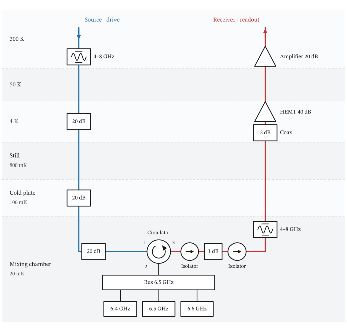
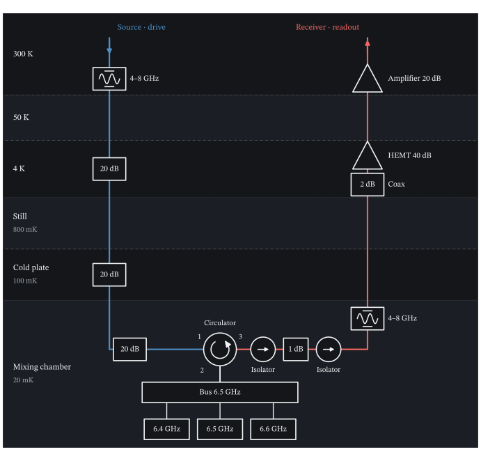
The drive descends the blue line; the reflected field returns along the red line. The three resonators couple to the bus at the mixing chamber. PDF

Measure the source-to-receiver response

Sweep the probe frequency between the exposed instrument ports. The chip has one coupling port but the source and receiver are separate, so the chip’s reflection appears in S21.

frequencies = np.linspace(6.34, 6.66, 401)
vna = VNA(readout_chip, ports=[drive, readout])
steady_state = vna.sweep(frequencies).s(readout, drive)

Plot S21

fig, magnitude_axis = plt.subplots(figsize=(6.4, 3.2), layout="constrained")
phase_axis = magnitude_axis.twinx()
phase_axis.grid(False)

magnitude_axis.plot(frequencies, 20 * np.log10(np.abs(steady_state)), color="#C92F33")
phase_axis.plot(frequencies, np.unwrap(np.angle(steady_state)) * 180 / np.pi, color="#246FA8", ls="--")

magnitude_axis.set(xlabel="Probe frequency (GHz)", ylabel=r"$|S_{21}|$ (dB)",
                   xlim=(frequencies[0], frequencies[-1]))
phase_axis.set(ylabel=r"Phase of $S_{21}$ (degrees)", yticks=[0, 180, 360, 540, 720, 900, 1080])
magnitude_axis.yaxis.label.set_color("#C92F33")
magnitude_axis.tick_params(axis="y", colors="#C92F33")
phase_axis.yaxis.label.set_color("#246FA8")
phase_axis.tick_params(axis="y", colors="#246FA8")
phase_axis.spines["right"].set_visible(True)
phase_axis.spines["right"].set_color("#246FA8")
magnitude_axis.spines["left"].set_color("#C92F33")
magnitude_axis.ticklabel_format(useOffset=False, axis="x")

fig.savefig("fridge_s21.svg")
plt.close(fig)

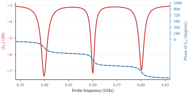
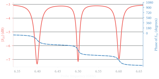
S21 at the room-temperature instrument ports. The 60 dB amplifier gain balances the 60 dB input attenuation; isolator and cable loss give an approximately −3 dB background. The three resonances add dips and phase windings. PDF

steady_state is the steady-state response of the full setup, including the bus, resonators, losses, filters, and amplifier gain. Added amplifier noise increases the fluctuation level but does not change this curve.

Sample a VNA trace

A sampled trace also needs the probe amplitude and the receiver integration time. Use an amplitude of 20 sqrt(photons/ns) at the source, before the 60 dB input attenuation. measure() computes the mean and noise spectra for this drive, and sample() then draws one complex IQ value at each probe frequency.

measurement = vna.measure(frequencies, amplitudes=20, input=drive, outputs=[readout])
short = measurement.sample(1, receiver=IQReceiver(integration_time=1_000_000), seed=19)
long = measurement.sample(1, receiver=IQReceiver(integration_time=100_000_000), seed=19)
np.testing.assert_allclose(measurement.ratio(readout), steady_state, atol=1e-10)

The two samples share one physical calculation. Increasing the integration time from 1 ms to 100 ms decreases the noise variance by approximately a factor of 100. The common random seed makes that change visible point by point.

Plot the sampled traces

fig, axes = plt.subplots(2, 2, figsize=(7.2, 4.6), sharex=True, sharey="row", layout="constrained")
fig.get_layout_engine().set(h_pad=0.02, w_pad=0.02)

steady_state_phase = np.unwrap(np.angle(steady_state))
for column, (samples, title) in enumerate(zip((short, long), ("1 ms integration", "100 ms integration"))):
    observed = samples.ratio(readout)[0]
    axes[0, column].plot(frequencies, 20 * np.log10(np.abs(observed)), ".", color="#C92F33", ms=2.6, alpha=0.7,
                         label="sampled IQ")
    axes[0, column].plot(frequencies, 20 * np.log10(np.abs(steady_state)), color="#16181C", lw=1.2, label="steady state")
    axes[1, column].plot(frequencies, (steady_state_phase + np.angle(observed / steady_state)) * 180 / np.pi, ".",
                         color="#C92F33", ms=2.6, alpha=0.7)
    axes[1, column].plot(frequencies, steady_state_phase * 180 / np.pi, color="#16181C", lw=1.2)
    axes[0, column].set_title(title)
    axes[1, column].set_xlabel("Probe frequency (GHz)")

axes[0, 0].set_ylabel("Output / input (dB)")
axes[1, 0].set(ylabel="Unwrapped phase (degrees)", yticks=[0, 360, 720, 1080])
axes[0, 1].legend(loc="lower right")
axes[1, 1].set_xlim(frequencies[0], frequencies[-1])

fig.savefig("fridge_measurement.svg")
plt.close(fig)

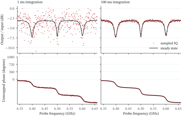
Solid lines show the steady state; red points are sampled IQ. The phase is shown on the steady-state curve’s unwrapped branch. Longer integration reduces the scatter in both magnitude and phase. PDF

The measurement also keeps the output noise spectrum. Use noise_spectrum() to report its power density at the receiver in dBm/Hz. Once you select an integration time, statistics() gives the IQ covariance and each source’s contribution to it.

statistics = measurement.statistics(receiver=IQReceiver(integration_time=1_000_000))
budget = statistics.noise_contributions(readout)
np.testing.assert_allclose(sum(budget.values()), statistics.covariance(readout), atol=1e-12)

noise_dbm_hz = measurement.noise_spectrum(readout, unit="dBm/Hz")
carrier_noise = noise_dbm_hz[..., len(measurement.noise_frequencies) // 2]
short_error = np.sqrt(np.mean(np.abs(short.ratio(readout)[0] - steady_state)**2))
long_error = np.sqrt(np.mean(np.abs(long.ratio(readout)[0] - steady_state)**2))

print(f"RESULT receiver_noise_dBm_per_Hz={np.mean(carrier_noise):.6f}")
print(f"RESULT short_complex_ratio_rmse={short_error:.6f}")
print(f"RESULT long_complex_ratio_rmse={long_error:.6f}")

Output:

RESULT receiver_noise_dBm_per_Hz=-132.467086
RESULT short_complex_ratio_rmse=0.175733
RESULT long_complex_ratio_rmse=0.017573

The same calculation gives the field and the mean photon number in each resonator. These include the input attenuation, the filters, the coupling through the bus, and the thermal noise that reaches the chip, and are independent of the receiver integration time.

r2 = resonators[1]
alpha = measurement.mode_amplitude(r2)
photons = measurement.photon_number(r2)
incoherent = photons - np.abs(alpha)**2

For this passive harmonic model, the coherent field scales with the source amplitude while the incoherent occupation stays fixed. At each frequency, the source amplitude for one stored photon on average is:

single_photon_amplitude = 20 * np.sqrt((1 - incoherent) / np.abs(alpha)**2)
peak = np.argmax(np.abs(alpha)**2)
one_photon = vna.measure(frequencies[peak], single_photon_amplitude[peak],
                        input=drive, outputs=[readout])
np.testing.assert_allclose(one_photon.photon_number(r2), 1.0, atol=1e-10)
print(f"RESULT r2_single_photon_amplitude={single_photon_amplitude[peak]:.2f}")

Output:

RESULT r2_single_photon_amplitude=144.04

The amplitude is in sqrt(photons/ns) at the source, and each frequency gives a separate drive setting. This rescaling requires a nonzero coherent response and an incoherent occupation below one. For nonlinear modes, solve again at the new drive amplitude. photon_number() still reports their full mean occupation from the density-matrix calculation.

Noise units and model limits

noise_spectrum() reports normally ordered fluctuations, without the coherent carrier and the detector vacuum. Its default unit is quanta. W/Hz and dBm/Hz use the absolute sideband frequency. The last array axis is the captured offset frequency.

Each source in statistics.noise_contributions() contributes a 2×2 IQ covariance in photons/ns, whose trace is the complex field variance. The sum includes the detector vacuum. device.correlations contains the interference between the input and the device field, and it can be negative.

Passive thermal_occupation and amplifier added_noise are constant quanta across the modeled band. Frequency sweeps still evaluate the filter transmission and the device response at each frequency. You can use linear eta and power gain instead of loss_db and gain_db.

The default offset grid spans ±0.1 GHz down to 1 Hz. If a narrower spectral feature needs more points, supply noise_frequencies=. Integration checks test the stored grid’s convergence and edge support but cannot find an unsampled feature. After changing the physical setup, call measure() again. Receiver time, digital filtering, calibration, and random draws use the captured arrays.

Stationary harmonic calculations use mode-space equations without a Fock cutoff, and nonlinear devices use the density-matrix solver. On a chip that conserves the total excitation and has more than 64 product states, the solver keeps the states with at most K excitations and warns which K it kept. Sampling describes stationary Gaussian field moments. Colored thermal noise into the chip needs an explicit dynamical filter or bath model. This setup does not include amplifier saturation, finite reverse isolation, or reverse amplifier noise.

Read a prepared qubit through the same line

A Rabi calculation can stop after state preparation. To describe an omitted readout stage, supply the mean output field for each qubit state before the downstream output components. The fridge then sets the receiver gain and noise.

This two-level qubit goes through one Rabi period. Its preparation is closed and uses sesolve, and the readout model below does not change that evolution.

from quchip import ChargeDrive, DuffingTransmon, IQReadout, QuantumSequence, Square

q = DuffingTransmon(freq=5.0, anharmonicity=-0.2, levels=2, label="q")
rabi_chip = Chip([q], frame="rotating")

xy = ChargeDrive(q, label="xy")
rabi_chip.wire(xy)

rabi = QuantumSequence(rabi_chip)
rabi.schedule(xy, envelope=Square(duration=40.0, amplitude=0.025), freq=5.0)

result = rabi.simulate(tlist=np.linspace(0, 40, 81))

detector = IQReadout.from_wiring(
    readout_chip, readout, frequency=6.5,
    means=[-0.01+0.001875j, 0.01-0.001875j],
    receiver=IQReceiver(integration_time=100_000),
)

measurement = result.measure(q, t=10.0)
shots = measurement.sample(1000, readout=detector, seed=7)

The supplied means are representative fields for outcomes 0 and 1, in \(1/\sqrt{\mathrm{ns}}\), before the selected channel’s downstream output components. They are defined at the output of the memoryless quantum network and summarize the readout interaction, so qubit populations alone cannot give them. The detector includes downstream filter, cable, and amplifier noise, plus heterodyne vacuum, integrated for 100 μs.

detector.contributions gives the source covariance budget.

Both panels use this detector, and a midpoint threshold classifies the IQ shots. The overlap gives an error of approximately 16% for each outcome. So the recorded Rabi curve spans approximately 0.16–0.84, while the quantum population spans 0–1. The qubit starts in |0⟩, so this floor is a detection error.

Plot the Rabi counts and IQ record

from scipy.special import ndtr

centers = np.stack((detector.means.real, detector.means.imag), axis=-1)
covariance = np.asarray(detector.iq_covariance[0])
direction = np.linalg.solve(covariance, centers[1]-centers[0])
threshold = direction @ centers.mean(axis=0)
sigma = np.sqrt(direction @ covariance @ direction)
excited_given_outcome = ndtr((centers @ direction-threshold)/sigma)

times = np.asarray(result.times)
probability = np.asarray(result.population(q, 1))
recorded_probability = excited_given_outcome[0]*(1-probability) + excited_given_outcome[1]*probability
fractions = []
for i, t in enumerate(times[::4]):
    record = result.measure(q, t=t).sample(256, readout=detector, seed=20+i)
    vectors = np.stack((record.iq.real, record.iq.imag), axis=-1)
    fractions.append(np.mean(vectors @ direction > threshold))

figure, axes = plt.subplots(1, 2, figsize=(8.8, 3.65), layout="constrained")
axes[0].plot(times, probability, color=ink, label="Born probability")
axes[0].plot(times, recorded_probability, color=red, label="After fridge + threshold")
axes[0].scatter(times[::4], fractions, s=18, color=blue, label="256 IQ shots", zorder=3)
axes[0].set(xlabel="Pulse duration (ns)", ylabel="Recorded excited fraction", xlim=(0, 40), ylim=(-0.04, 1.1))
axes[0].legend(fontsize=8, loc="upper right")
for outcome, color in enumerate((blue, red)):
    points = shots.iq[shots.physical_indices == outcome]
    axes[1].scatter(points.real, points.imag, s=6, alpha=0.65, color=color,
                    edgecolors="none", label=f"Outcome {outcome}")
    axes[1].plot(centers[outcome, 0], centers[outcome, 1], "+", color=ink, ms=9, mew=1.4)

span = np.max(np.abs(centers)) + 4*np.sqrt(np.max(np.diag(covariance)))
tangent = np.array([-direction[1], direction[0]]) / np.linalg.norm(direction)
boundary = centers.mean(axis=0)[:, None] + tangent[:, None]*np.array([-span, span])
axes[1].plot(*boundary, color=muted, ls="--", lw=1, label="Threshold")
axes[1].set(xlabel=r"I ($1/\sqrt{\mathrm{ns}}$)", ylabel=r"Q ($1/\sqrt{\mathrm{ns}}$)",
            xlim=(-span, span), ylim=(-span, span))
axes[1].set_aspect("equal", adjustable="box")
axes[1].legend(fontsize=8, loc="upper center", ncol=2)
figure.suptitle(r"Fridge output at 6.5 GHz $\cdot$ 100 $\mu$s integration", fontsize=12)

figure.savefig("terminal_rabi.svg")
plt.close(figure)

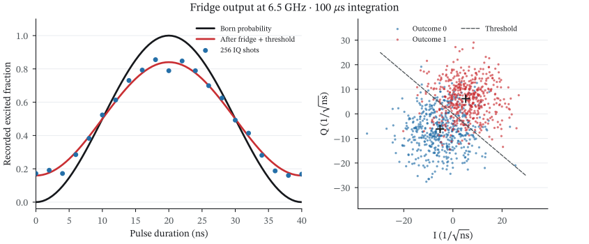
The output chain rotates and amplifies the supplied fields and broadens their IQ distributions. Colors mark physical outcomes; the threshold determines the recorded labels. PDF

result.measure() works with kets or density matrices and uses the local energy bases that the simulation saved. Pass several devices for joint outcomes, or pass t= for an exact saved state. Final measurement works with states="final". Different measurement times represent separate terminated experiments.

If a simulation already includes the fridge, result.iq_readout(...) reuses the wiring saved with it. IQReadout.from_wiring(...) resolves the current wiring without quantum evolution. Both assume coherent fields at the quantum-network output and vacuum in unspecified input channels. Thermal input fields and correlations with the devices need a field calculation or a detector calibration that includes them. In that case, use a calibrated IQReadout(means, iq_covariance) directly, and do not add the same apparatus noise again.

For lifetime design, continue with Purcell filtering and T1. For pulse shaping and cavity depletion, see pulses, leakage, and readout.