

Gradients and parameter fitting
Differentiate dressed observables and pulse responses, and use JAX gradients to fit measured spectroscopy.
Gradients of spectral observables
A scalar fitting objective has a gradient and a vector residual has a Jacobian, and
both go through the same public Chip.with_params() call.
The second observable is the coefficient of \(Z n_r\), with \(Z=|0\rangle\langle0|-|1\rangle\langle1|\) and \(\chi_Z=-\mathrm{dispersive\_shift}/2\). The scalar method returns the full pull \(E_{11}-E_{10}-E_{01}+E_{00}\).
import jax
import jax.numpy as jnp
import numpy as np

from quchip import Capacitive, Chip, DuffingTransmon, Resonator

q = DuffingTransmon(freq=5.0, anharmonicity=-0.25, levels=4, label="q")
r = Resonator(freq=7.0, levels=4, label="r")

chip = Chip(
    [q, r],
    [Capacitive(q, r, g=0.05, label="qr")],
    frame="rotating",
    backend="dynamiqs",
)
Define a scalar fitting objective and a vector residual. jax.grad gives the loss
gradient, and jax.jacrev gives the observable’s Jacobian. Sweep the coupling to compare
the resolved curve with its local tangent.
names = ["q.freq", "q.anharmonicity", "qr.g"]
theta = jnp.array([5.0, -0.25, 0.05])
target = jnp.array([5.05, 0.0010])  # [f01, chi_z] in GHz


def observables(th):
    c = chip.with_params(dict(zip(names, th)))
    chi_z = -c.dispersive_shift("q", "r") / 2
    return jnp.stack([jnp.asarray(c.freq("q")), jnp.asarray(chi_z)])


def residual(th):
    return observables(th) - target


def loss(th):
    return jnp.sum(residual(th) ** 2)


static_gradient = jax.grad(loss)(theta)
static_jacobian = jax.jacrev(residual)(theta)

coupling_values = jnp.linspace(0.02, 0.08, 61)
observable_sweep = jax.vmap(
    lambda coupling: observables(theta.at[2].set(coupling))
)(coupling_values)
coupling_tangent = observables(theta) + (
    coupling_values[:, None] - theta[2]
) * static_jacobian[:, 2]
Plotting code
import shutil
import matplotlib.pyplot as plt

plt.style.use("../docs/_static/quchip.mplstyle")
plt.rcParams["text.usetex"] = bool(shutil.which("latex"))

static_figure, static_axes = plt.subplots(1, 2, figsize=(9.2, 3.8), layout="constrained")
for observable_index, (axis, ylabel, scale) in enumerate(
    zip(
        static_axes,
        (r"$f_{01}$ (GHz)", r"$\chi_Z$ (MHz)"),
        (1.0, 1.0e3),
        strict=True,
    )
):
    axis.plot(
        1.0e3 * coupling_values,
        scale * observable_sweep[:, observable_index],
        color="#C92F33",
        linewidth=2.2,
        label="quchip sweep",
    )
    axis.plot(
        1.0e3 * coupling_values,
        scale * coupling_tangent[:, observable_index],
        color="#16181C",
        linestyle="--",
        linewidth=1.4,
        label="local tangent",
    )
    axis.plot(
        1.0e3 * theta[2],
        scale * observables(theta)[observable_index],
        marker="o",
        color="#16181C",
        markeredgecolor="white",
        markersize=7,
        linestyle="none",
    )
    axis.set(xlabel=r"Capacitive coupling $g$ (MHz)", ylabel=ylabel)

static_axes[0].legend()

static_figure_path = "../docs/images/differentiate_static_slope.svg"
static_figure.savefig(static_figure_path)
plt.show()
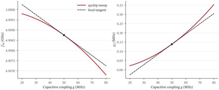
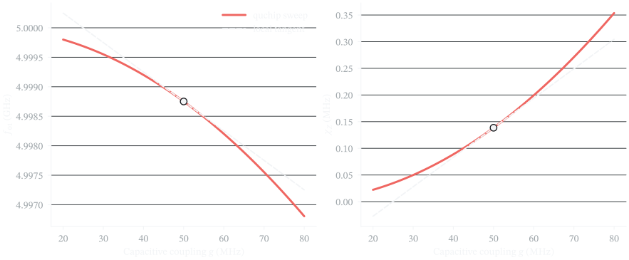
The black point is where jax.jacrev evaluates the slope. The dispersive shift
bends away from its tangent faster than \(f_{01}\) over this range.
Fit measured spectroscopy
Stefanski et al. fitted a fluxonium spectrum to get \(E_C\), \(E_J\), and \(E_L\). Their paper and analysis repository publish the extracted frequencies and fitted parameters. Here we start away from those parameters and minimize a differentiable quchip loss.
Every eighth measurement goes into the fit, and the points between them are held out. The plotted model uses its own 351-point flux grid.
Load the published data and select fit points
import csv
import io
import json
from urllib.request import urlopen

from scipy.optimize import minimize

from quchip import Fluxonium

paper_data_root = (
    "https://raw.githubusercontent.com/AndersenQubitLab/"
    "FPA-RO-experimental/57dc268dd048d1372db082c3ddd97a04871580bf"
)

with urlopen(f"{paper_data_root}/processed_data_fx8.csv") as response:  # noqa: S310
    spectrum_rows = list(
        csv.DictReader(io.StringIO(response.read().decode("utf-8")))
    )

published_values = np.asarray(
    [float(spectrum_rows[index]["energy_params"]) for index in range(5)]
)
published_energies = published_values[[3, 2, 4]]  # E_C, E_J, E_L

measured_flux_all = np.asarray(
    [float(row["phi_ext_qubit"]) for row in spectrum_rows if row["phi_ext_qubit"]]
)
measured_f01_all = np.asarray(
    [float(row["qubit_freq"]) for row in spectrum_rows if row["qubit_freq"]]
)
paper_window = measured_flux_all <= 0.85
measured_flux = measured_flux_all[paper_window]
measured_f01 = measured_f01_all[paper_window]

training_indices = np.arange(0, measured_flux.size, 8)
holdout_mask = np.ones(measured_flux.size, dtype=bool)
holdout_mask[training_indices] = False
training_flux = jnp.asarray(measured_flux[training_indices])
training_f01 = jnp.asarray(measured_f01[training_indices])
The optimization model uses a 160-point phase grid. Logarithmic coordinates keep the three circuit energies positive and put them on comparable numerical scales.
fit_q = Fluxonium(
    E_C=0.72,
    E_J=4.4,
    E_L=0.68,
    phi_ext=0.5,
    levels=4,
    num_basis=160,
    phi_max=5.0 * np.pi,
    basis="eigen",
    label="q",
)
fit_chip = Chip(
    [fit_q],
    [],
    basis="eigen",
    frame="lab",
    backend="dynamiqs",
)

energy_scale = jnp.asarray([1.0, 4.0, 1.0])
initial_energies = np.asarray([0.72, 4.4, 0.68])
initial_coordinates = jnp.log(jnp.asarray(initial_energies) / energy_scale)


def energies_from_coordinates(coordinates):
    return energy_scale * jnp.exp(coordinates)


def fluxonium_f01(energies, phi_ext):
    point = fit_chip.with_params(
        {
            "q.E_C": energies[0],
            "q.E_J": energies[1],
            "q.E_L": energies[2],
            "q.phi_ext": phi_ext,
        }
    )
    return point.freq("q")


def spectrum_prediction(coordinates, flux):
    energies = energies_from_coordinates(coordinates)
    return jax.vmap(lambda phi: fluxonium_f01(energies, phi))(flux)
Fit a smooth robust loss, which limits the influence of spectroscopy outliers, with SciPy’s bounded optimizer. JAX supplies the loss gradient.
def pseudo_huber(residual):
    return 2.0 * (jnp.sqrt(1.0 + residual**2) - 1.0)


def experimental_loss(coordinates):
    residual_mhz = 1.0e3 * (
        spectrum_prediction(coordinates, training_flux) - training_f01
    )
    return jnp.mean(pseudo_huber(residual_mhz / 3.0))


compiled_loss_and_gradient = jax.jit(jax.value_and_grad(experimental_loss))
loss_history = []


def scipy_objective(coordinates):
    value, gradient = compiled_loss_and_gradient(jnp.asarray(coordinates))
    return float(value), np.asarray(gradient, dtype=float)


fit = minimize(
    scipy_objective,
    np.asarray(initial_coordinates),
    method="L-BFGS-B",
    jac=True,
    bounds=[
        (np.log(0.3), np.log(1.5)),
        (np.log(2.0 / 4.0), np.log(6.0 / 4.0)),
        (np.log(0.3), np.log(1.5)),
    ],
    callback=lambda coordinates: loss_history.append(
        scipy_objective(coordinates)[0]
    ),
    options={"maxiter": 160, "ftol": 1.0e-12, "gtol": 1.0e-9},
)

recovered_energies = np.asarray(
    energies_from_coordinates(jnp.asarray(fit.x)),
    dtype=float,
)
The evaluation starts from a new 351-point model grid. After that forward calculation, interpolation puts the model at the held-out measurement coordinates for the residual check.
model_flux = jnp.linspace(0.5, 0.85, 351)
model_f01 = np.asarray(spectrum_prediction(jnp.asarray(fit.x), model_flux))
predicted_at_measurements = np.interp(
    measured_flux,
    np.asarray(model_flux),
    model_f01,
)
holdout_residual_mhz = 1.0e3 * (
    predicted_at_measurements[holdout_mask] - measured_f01[holdout_mask]
)
Plotting code
from matplotlib.ticker import LogLocator, MaxNLocator, NullFormatter, ScalarFormatter

fit_figure, (fit_axis, history_axis) = plt.subplots(
    1,
    2,
    figsize=(10.0, 4.2),
    layout="constrained",
)
fit_axis.scatter(
    measured_flux[holdout_mask],
    measured_f01[holdout_mask],
    s=13,
    color="#9AA0A8",
    label="held out",
)
fit_axis.scatter(
    measured_flux[training_indices],
    measured_f01[training_indices],
    s=23,
    color="#C92F33",
    marker="x",
    label="fit points",
)
fit_axis.plot(model_flux, model_f01, color="#246FA8", linewidth=2.2, label="quchip")
fit_axis.set(
    xlabel=r"External flux $\Phi_{\mathrm{ext}}/\Phi_0$",
    ylabel=r"$f_{01}$ (GHz)",
)
fit_axis.legend()

history_axis.semilogy(loss_history, color="#C92F33", linewidth=2.0)
history_axis.set(xlabel="Optimizer iteration", ylabel="Spectrum loss")
history_axis.yaxis.set_major_locator(LogLocator(subs=(1.0, 2.0, 5.0)))
history_axis.yaxis.set_major_formatter(ScalarFormatter())
history_axis.yaxis.set_minor_formatter(NullFormatter())
history_axis.xaxis.set_major_locator(MaxNLocator(integer=True))

experimental_fit_path = "../docs/images/differentiate_fluxonium_fit.svg"
fit_figure.savefig(experimental_fit_path)
plt.show()
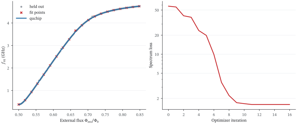
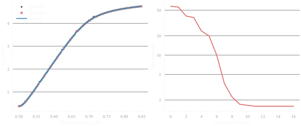
Twenty measurements determine the loss. The remaining 133 points test the recovered spectrum.
Numerical record
experimental_fit_receipt = {
    "fit_success": bool(fit.success),
    "iterations": int(fit.nit),
    "training_points": len(training_indices),
    "holdout_points": int(holdout_mask.sum()),
    "published_E_C_E_J_E_L": published_energies.tolist(),
    "initial_E_C_E_J_E_L": initial_energies.tolist(),
    "recovered_E_C_E_J_E_L": recovered_energies.tolist(),
    "relative_parameter_error": (
        (recovered_energies - published_energies) / published_energies
    ).tolist(),
    "holdout_median_absolute_error_mhz": float(
        np.median(np.abs(holdout_residual_mhz))
    ),
    "holdout_rmse_mhz": float(np.sqrt(np.mean(holdout_residual_mhz**2))),
}

print(
    "RESULT experimental_statics="
    + json.dumps(experimental_fit_receipt, sort_keys=True, separators=(",", ":"))
)
Output:
RESULT experimental_statics={"fit_success":true,"holdout_median_absolute_error_mhz":0.8806168653689994,"holdout_points":133,"holdout_rmse_mhz":6.967105550535916,"initial_E_C_E_J_E_L":[0.72,4.4,0.68],"iterations":17,"published_E_C_E_J_E_L":[0.8652719648666846,3.8217399868188027,0.8215798519627777],"recovered_E_C_E_J_E_L":[0.8704199134602235,3.8203629719093892,0.8208603213336979],"relative_parameter_error":[0.005949515068747334,-0.00036031098770789575,-0.0008757890390822424],"training_points":20}
The recovered circuit energies are within \(0.6\%\) of the authors’ values. The few large spectroscopy residuals stay in the holdout RMSE, and the median error is \(0.88\) MHz. This section fits the isolated fluxonium spectrum, while the paper’s full fit also included the coupled readout resonator.
Differentiate a pulse response
Differentiate the final excited-state population with respect to pulse amplitude, Gaussian shape, and detuning.
The dynamiqs backend keeps these declared parameters differentiable through
the time-domain solve. Install the backend with
pip install 'quchip[dynamiqs]'.
from quchip import RWA, ChargeDrive, Chip, DuffingTransmon, Gaussian, QuantumSequence

amplitude0 = 0.029
frequency0 = 5.0
sigmas0 = 3.0

qubit = DuffingTransmon(
    freq=frequency0,
    anharmonicity=-0.30,
    levels=3,
    label="q",
)

chip = Chip(
    [qubit],
    frame="rotating",
    approximation=RWA(),
    backend="dynamiqs",
)
drive = ChargeDrive(qubit, label="xy")
_ = chip.wire(drive)

sequence = QuantumSequence(chip)
_ = sequence.schedule(
    drive,
    envelope=Gaussian(duration=40.0, sigmas=sigmas0, amplitude=amplitude0),
    freq=frequency0,
)

times = jnp.linspace(0.0, 60.0, 121)
original_parameters = dict(sequence.parameters)
One unit in the perturbation vector means \(1\%\) in pulse amplitude, \(1\%\) in
the Gaussian parameter \(N_\sigma\), or \(1\) MHz in pulse detuning. quchip defines
\(\sigma=\mathrm{duration}/(2N_\sigma)\). So increasing \(N_\sigma\) by \(1\%\)
narrows the physical Gaussian width by approximately \(1\%\). The derivatives
predict changes in final population on these three scales. jax.value_and_grad
returns the population and its derivatives together.
parameter_paths = ("pulse.0.amplitude", "pulse.0.sigmas", "pulse.0.freq")
perturbation_labels = (
    r"amplitude (+1\%)",
    r"$N_\sigma$ (+1\%; $\sigma$ $-$1\%)",
    "detuning (+1 MHz)",
)


def final_population(perturbation):
    rebound = sequence.with_params(
        {
            "pulse.0.amplitude": amplitude0 * (1.0 + 0.01 * perturbation[0]),
            "pulse.0.sigmas": sigmas0 * (1.0 + 0.01 * perturbation[1]),
            "pulse.0.freq": frequency0 + perturbation[2] * 1.0e-3,
        }
    )
    result = rebound.simulate(
        tlist=times,
        initial_state={"q": 0},
        partition=False,
    )
    return jnp.real(result.population("q", level=1)[-1])


origin = jnp.zeros(3)
population0, gradient = jax.jit(jax.value_and_grad(final_population))(origin)
At this operating point, increasing amplitude or detuning raises the final population, and a narrower Gaussian lowers it.
Plotting code
impact = np.asarray(gradient) * 1000

figure, axis = plt.subplots(figsize=(7.2, 2.8), layout="constrained")
axis.barh(perturbation_labels, impact, height=0.55,
          color=["#C92F33" if value >= 0 else "#246FA8" for value in impact])
axis.axvline(0, color="#16181C", lw=0.8)
axis.set(xlabel=r"Predicted $\Delta P(q=1)$ ($\times 10^{-3}$)")
axis.invert_yaxis()
axis.grid(False, axis="y")
axis.grid(True, axis="x")
axis.spines["left"].set_visible(False)
axis.tick_params(axis="y", length=0)

figure_path = "../docs/images/differentiate_a_driven_chip.svg"
figure.savefig(figure_path)
plt.show()
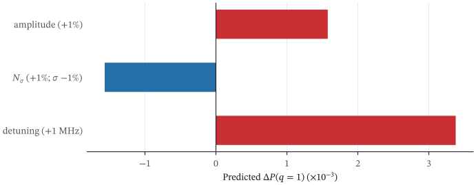
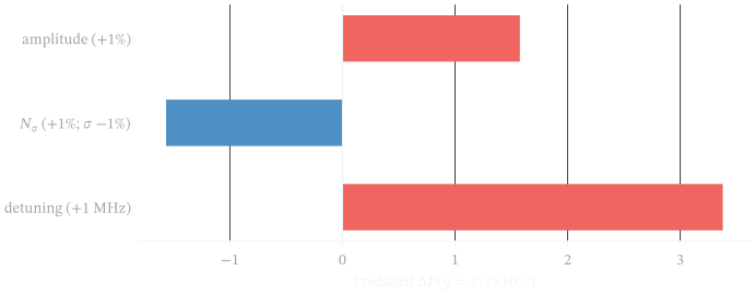
Each bar predicts the population change for the perturbation named on its axis.
Advanced: share calibration parameters across three experiments
Combine three pulse experiments with a shared qubit frequency, amplitude scale, and carrier correction. Their durations and nominal detunings stay fixed.
experiment_settings = (
    (18.0, 0.020, -0.004),
    (28.0, 0.026, 0.000),
    (40.0, 0.029, 0.004),
)
experiments = []
for duration, amplitude, carrier_offset in experiment_settings:
    experiment = QuantumSequence(chip)
    experiment.schedule(
        drive,
        envelope=Gaussian(duration=duration, sigmas=3.0, amplitude=amplitude),
        freq=frequency0 + carrier_offset,
    )
    experiments.append(experiment)

shared_names = ("q.freq", "amplitude scale", "carrier correction")
shared_origin = jnp.array([frequency0, 1.0, 0.0])
multi_times = jnp.linspace(0.0, 60.0, 81)
Rebind the shared parameters across the three schedules and collect their final populations.
def experiment_outputs(shared):
    qubit_frequency, amplitude_scale, carrier_correction = shared
    values = []
    for experiment, (_, nominal_amplitude, nominal_offset) in zip(
        experiments, experiment_settings
    ):
        rebound = experiment.with_params(
            {
                "q.freq": qubit_frequency,
                "pulse.0.amplitude": nominal_amplitude * amplitude_scale,
                "pulse.0.freq": frequency0 + nominal_offset + carrier_correction,
            }
        )
        result = rebound.simulate(
            tlist=multi_times,
            initial_state={"q": 0},
            partition=False,
        )
        values.append(jnp.real(result.population("q", level=1)[-1]))
    return jnp.stack(values)
Combine the experiment residuals into one weighted calibration loss.
reference_outputs = experiment_outputs(shared_origin)
multi_targets = jax.lax.stop_gradient(
    reference_outputs + jnp.array([0.010, -0.015, 0.005])
)
experiment_weights = jnp.array([1.0, 2.0, 0.5])


def multi_residual(shared):
    return experiment_outputs(shared) - multi_targets


def multi_loss(shared):
    return jnp.sum(experiment_weights * multi_residual(shared) ** 2)
The Jacobian has one row for each experiment and one column for each shared parameter.
multi_jacobian = jax.jacrev(multi_residual)(shared_origin)
multi_loss_gradient = jax.grad(multi_loss)(shared_origin)
Use the Jacobian to see which experiment constrains each parameter, and the loss gradient for an optimization step.
Numerical record
reference_result = sequence.simulate(
    tlist=times,
    initial_state={"q": 0},
    partition=False,
)

gradient_receipt = {
    "backend": "dynamiqs",
    "base_population": float(population0),
    "figure": figure_path,
    "first_order_only": True,
    "fixed_structure_during_trace": True,
    "gradient_per_reference_perturbation": {
        path: float(value) for path, value in zip(parameter_paths, gradient)
    },
    "multi_sequence_count": len(experiments),
    "multi_sequence_jacobian_shape": list(multi_jacobian.shape),
    "multi_sequence_loss_gradient": [float(value) for value in multi_loss_gradient],
    "original_sequence_unchanged": dict(sequence.parameters) == original_parameters,
    "parameter_paths": list(parameter_paths),
    "solver": reference_result.solver,
}

print(f"RESULT gradient={json.dumps(gradient_receipt, sort_keys=True, separators=(',', ':'))}")
Output:
RESULT gradient={"backend":"dynamiqs","base_population":0.9955197597010083,"figure":"../docs/images/differentiate_a_driven_chip.svg","first_order_only":true,"fixed_structure_during_trace":true,"gradient_per_reference_perturbation":{"pulse.0.amplitude":0.0015756847934132964,"pulse.0.freq":0.0033782484014230805,"pulse.0.sigmas":-0.0015669142083585888},"multi_sequence_count":3,"multi_sequence_jacobian_shape":[3,3],"multi_sequence_loss_gradient":[-0.09312829969383697,0.045324706488043695,0.093128299693837],"original_sequence_unchanged":true,"parameter_paths":["pulse.0.amplitude","pulse.0.sigmas","pulse.0.freq"],"solver":"sesolve"}
Gradient assumptions and limits
The traced calculation keeps the device graph, Hilbert-space dimensions, and RWA band selection fixed. dynamiqs supports this automatic-differentiation path. QuTiP remains available for ordinary solves and sweeps but does not give gradients. Near degenerate subspaces, be careful with eigenvector derivatives. Gradients inherit the solver tolerances, local-basis truncation, frame, approximation, and loss scaling of the forward calculation.