Pulses, leakage, and readout

How does pulse duration change leakage, and how does the qubit state appear in resonator readout? Use one coupled model for both experiments. Frequencies are in GHz and times in ns.

Declare the chip

The transmon couples to a 6.8 GHz resonator with a 1 MHz linewidth. Separate charge lines address the qubit and the readout.

import numpy as np
from scipy import integrate
from quchip import (
    RWA, Capacitive, ChargeDrive, Chip, DuffingTransmon,
    Gaussian, GaussianEdge, QuantumSequence, Resonator,
)

qubit = DuffingTransmon(freq=5.0, anharmonicity=-0.30, levels=6, label="q")
readout = Resonator(freq=6.8, levels=10, internal_quality_factor=6800, label="r")
chip = Chip(
    [qubit, readout], [Capacitive(qubit, readout, g=0.060, label="qr")],
    frame="rotating", approximation=RWA(),
)

qubit_line = ChargeDrive(qubit, label="qubit-charge")
readout_line = ChargeDrive(readout, label="readout-charge")
_ = chip.wire(qubit_line, readout_line)

Compare a short and a long qubit pulse

Both Gaussians have the same nominal π area. The short pulse’s spectral width is comparable to the separation between the dressed 0→1 and 1→2 transitions, so the four-times-longer pulse is more selective.

f01 = float(chip.freq(qubit))
f12 = float(chip.transition_frequency(qubit, 1, 2))
drive_durations = 3 / (np.pi * abs(f12 - f01)) * np.array([1.0, 4.0])


def pi_gaussian(duration):
    unit_pulse = Gaussian(duration=duration, sigmas=3.0, amplitude=1.0)
    grid = np.linspace(0, duration, 20001)
    area = integrate.trapezoid(np.asarray(unit_pulse.value(grid)).real, grid)
    return Gaussian(duration=duration, sigmas=3.0, amplitude=0.5 / area)


drive_pulses = [pi_gaussian(duration) for duration in drive_durations]

Schedule the short pulse, then change its duration and amplitude together. Each batch member starts in dressed |0,0⟩ and uses the same time grid.

drive_sequence = QuantumSequence(chip)
drive = drive_sequence.schedule(qubit_line, envelope=drive_pulses[0], freq=f01)
drive_times = np.linspace(0, drive_durations[-1], 601)

drive_batch = drive_sequence.simulate_batch(
    drive_sequence.zip(
        drive.vary("duration", drive_durations),
        drive.vary("amplitude", [pulse.amplitude for pulse in drive_pulses]),
    ),
    tlist=drive_times,
    initial_state=chip.state({qubit: 0, readout: 0}),
    progress=False,
)

Read the populations of |0⟩, |1⟩, and |2⟩. The arrays are indexed by (level, pulse, time).

drive_populations = np.asarray([
    drive_batch.population(qubit, level) for level in range(3)
]).real

Plot the envelopes and populations

import shutil
import matplotlib.pyplot as plt

plt.style.use("../docs/_static/quchip.mplstyle")
plt.rcParams["text.usetex"] = bool(shutil.which("latex"))

colors = ("#16181C", "#246FA8", "#C92F33")

figure, axes = plt.subplots(2, 1, figsize=(6.6, 5.2), sharex=True, layout="constrained")
for index, (axis, name, envelope) in enumerate(zip(axes, ("Short", "Long"), drive_pulses)):
    for level, color in enumerate(colors):
        axis.plot(drive_times, drive_populations[level, index], color=color,
                  lw=1.8, label=fr"$P(|{level}\rangle)$")
    pulse_axis = axis.twinx()
    pulse_axis.plot(drive_times, np.where(drive_times <= envelope.duration,
                    envelope.sample(drive_times, real=True), 0.0),
                    color="#6D7277", ls="--", lw=1.2)
    pulse_axis.set(ylabel="Envelope (GHz)", ylim=(0, 1.1 * drive_pulses[0].amplitude))
    pulse_axis.spines["right"].set_visible(True)
    pulse_axis.spines["right"].set_color("#6D7277")
    pulse_axis.yaxis.label.set_color("#6D7277")
    pulse_axis.tick_params(axis="y", colors="#6D7277")
    axis.set(ylabel="Population", ylim=(-0.02, 1.02), xlim=(0, drive_times[-1]))
    axis.set_title(fr"{name} Gaussian $\cdot$ {envelope.duration:.2f} ns")

axes[0].legend(ncol=3, loc="upper right", fontsize=9)
axes[1].set_xlabel("Time (ns)")

figure.savefig("../docs/images/hello_qubit_drive_leakage.svg")

figure.savefig("../docs/images/hello_qubit_drive_leakage.png")
plt.show()

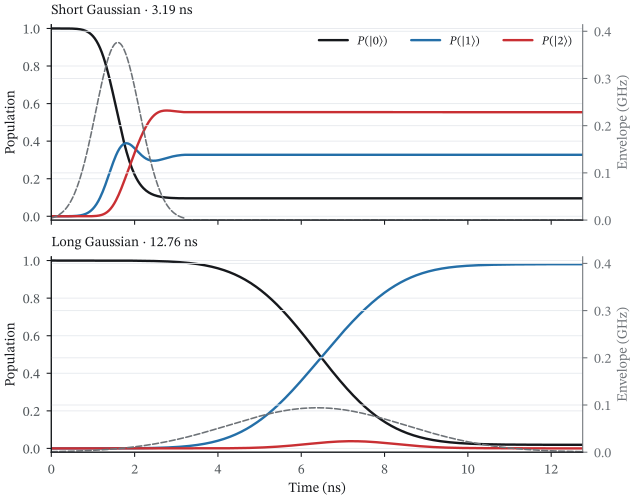
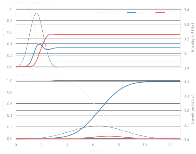
Dashed grey curves show the drive envelopes. The short pulse populates |2⟩; the longer pulse leaves most population in |1⟩. PDF

for index, name in enumerate(("Short", "Long")):
    print(
        f"{name}: final P1 = {drive_populations[1, index, -1]:.1%}; "
        f"peak P2 = {drive_populations[2, index].max():.1%}"
    )

Output:

Short: final P1 = 32.7%; peak P2 = 56.3%
Long: final P1 = 98.1%; peak P2 = 3.8%

Equal pulse area does not guarantee equal inversion in a multilevel system. The smaller peak P2 shows why the longer pulse comes closer to the target.

Read out the prepared qubit state

Now drive the resonator, whose frequency depends on the qubit state. Use a tone halfway between the dressed resonances for qubit states |0⟩ and |1⟩, with the same RWA Hamiltonian as the simulation. To see the IQ response in the drive frame, set reference_freq to the carrier.

readout_dressed = chip.resolve(frame="lab").dress()
readout_energies = readout_dressed.dressed_eigenvalues
readout_frequencies = [
    float(readout_energies[(level, 1)] - readout_energies[(level, 0)])
    for level in (0, 1)
]
readout_carrier = np.mean(readout_frequencies)
readout.reference_freq = readout_carrier

readout_pulse = GaussianEdge(duration=900.0, edge_duration=40.0, sigmas=3, amplitude=0.0012)
readout_sequence = QuantumSequence(chip)
_ = readout_sequence.schedule(readout_line, envelope=readout_pulse, freq=readout_carrier)

Apply the same pulse to separately prepared dressed |0,0⟩ and |1,0⟩ states. As these are new preparations, the readout comparison does not inherit the previous experiment’s leakage. Follow the two IQ pointers during the 900 ns readout pulse.

readout_times = np.linspace(0, 900, 181)

readout_batch = readout_sequence.simulate_batch(
    readout_sequence.vary(
        "initial_state",
        [readout_dressed.eigenstates[readout_dressed.state_map[(level, 0)]]
         for level in (0, 1)],
        name="prepared_qubit",
    ),
    tlist=readout_times,
    e_ops=chip.e_ops(r="a"),
    progress=False,
)

expect("r") returns the requested α(t) = ⟨a⟩. Compare the two complex responses and their separation over time.

alpha = np.asarray(readout_batch.expect("r"), dtype=complex)
iq_separation = np.abs(alpha[0] - alpha[1])

Plot the readout pulse and IQ response

figure, (time_axis, iq_axis) = plt.subplots(2, 1, figsize=(6.0, 6.4),
                                         height_ratios=(0.55, 2.2), layout="constrained")

time_axis.plot(readout_times, 1000 * readout_pulse.sample(readout_times, real=True),
               color="#16181C", lw=1.8)
time_axis.set(xlabel="Time (ns)", ylabel="Envelope (MHz)", xlim=(0, 900), yticks=[0, 1.2])
time_axis.set_title("(a) Readout pulse")

for level, color in enumerate(("#246FA8", "#C92F33")):
    path = alpha[level]
    iq_axis.plot(path.real, path.imag, color=color, lw=1.8,
                 label=fr"Prepared $|{level}\rangle$")
    for time in (100, 300, 900):
        point = path[np.searchsorted(readout_times, time)]
        iq_axis.plot(point.real, point.imag, "o", color=color, ms=5)
        offset = {100: (-8, 6 if level == 0 else -14), 300: (10, 7 if level == 0 else -15), 900: (8, 6)}
        iq_axis.annotate(f"{time} ns", (point.real, point.imag), xytext=offset[time],
                         textcoords="offset points", ha="right" if time == 100 else "left",
                         color=color, fontsize=9)
    start, end = path[90], path[96]
    iq_axis.annotate("", (end.real, end.imag), (start.real, start.imag),
                     arrowprops={"arrowstyle": "->", "color": color, "lw": 1.8})

iq_axis.plot(0, 0, "+", color="#16181C", ms=8)
iq_axis.set(xlabel=r"$\mathrm{Re}\,\alpha$", ylabel=r"$\mathrm{Im}\,\alpha$",
            xlim=(1.15 * alpha.real.min(), 0.22), ylim=(1.2 * alpha.imag.min(), 1.2 * alpha.imag.max()))
iq_axis.set_title("(b) Intracavity IQ in the drive frame")
iq_axis.set_aspect("equal", adjustable="box")
iq_axis.legend(fontsize=9, loc="upper right")

figure.savefig("../docs/images/hello_dispersive_readout_iq.svg")

figure.savefig("../docs/images/hello_dispersive_readout_iq.png")
plt.show()

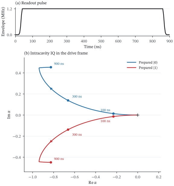
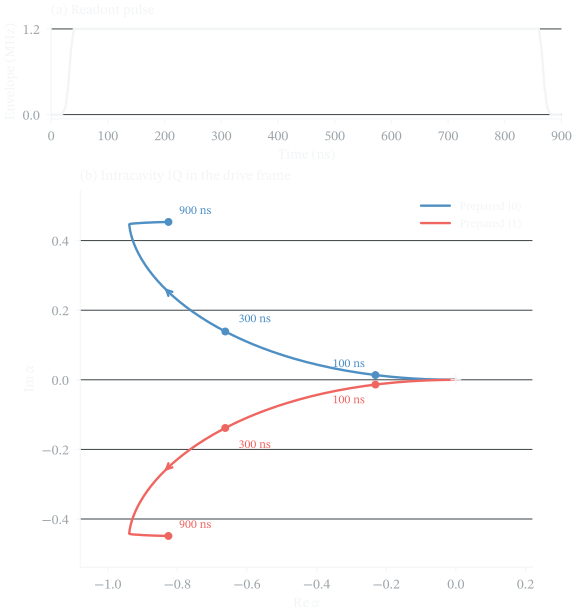
Above: the readout pulse envelope. Below: the IQ pointers traced during readout, with time markers and arrows showing the direction of motion. The cross marks zero field. PDF

The same drive produces distinguishable mean fields for the two qubit states, as intracavity responses rather than a single-shot fidelity estimate.

Numerical checks and record

import json

for result in (*drive_batch, *readout_batch):
    top_levels = result.check_truncation(threshold=1.0)
    assert max(top_levels.values()) < 1e-3

drive_receipt = {
    "final_p1": dict(zip(("short", "long"), drive_populations[1, :, -1])),
    "peak_p2": dict(zip(("short", "long"), drive_populations[2].max(axis=-1))),
}
readout_receipt = {
    "conditional_resonator_frequencies_ghz": readout_frequencies,
    "final_iq_separation": float(iq_separation[-1]),
    "solver": readout_batch[0].solver,
}
print(f"RESULT drive={json.dumps(drive_receipt, sort_keys=True)}")
print(f"RESULT readout={json.dumps(readout_receipt, sort_keys=True)}")

Output:

RESULT drive={"final_p1": {"long": 0.9808186959428491, "short": 0.3274130996871264}, "peak_p2": {"long": 0.03843070489891596, "short": 0.5631356326693838}}
RESULT readout={"conditional_resonator_frequencies_ghz": [6.801997782702374, 6.801428548310606], "final_iq_separation": 0.9021929173380938, "solver": "mesolve"}

Empty the resonator after readout

When a readout pulse stops, photons remain and decay. A CLEAR pulse adds loading and depletion segments that build up and remove the coherent field faster.

Use the filtered circuit from the T1 guide: a 5 GHz transmon, a 7 GHz readout resonator, and a 7.02 GHz Purcell filter. The line couples to the filter. Both pulses use the same 7.004945 GHz carrier, a weak-drive estimate of the conditional response midpoint that includes the lossy filter. Use that carrier as the IQ reference too.

from quchip import Capacitive, Chip, DuffingTransmon, PortNetwork, QuantumSequence, Resonator, RWA, Square

clear_carrier = 7.004945346
clear_q = DuffingTransmon(freq=5.0, anharmonicity=-0.2, levels=3, T1=60_000, label="q")
clear_r = Resonator(freq=7.0, levels=4, internal_quality_factor=200_000, label="r")
clear_f = Resonator(freq=7.02, levels=2, internal_quality_factor=100_000, label="f")
clear_r.reference_freq = clear_carrier

clear_network = PortNetwork(label="feedline")
filter_rate = 2 * np.pi * 0.230
chip_port = clear_network.expose("feedline", at=clear_network.port("feed", target=clear_f, rate=filter_rate))

clear_chip = Chip(
    [clear_q, clear_r, clear_f],
    [Capacitive(clear_q, clear_r, g=0.105, label="qr"),
     Capacitive(clear_r, clear_f, g=0.007696696, label="rf")],
    port_network=clear_network, frame=clear_carrier, approximation=RWA(),
)

Both pulses start at 100 ns and use the same carrier and hold amplitude (in √photons/ns). The square pulse stops at 900 ns. CLEAR uses two loading segments, a hold, and then two depletion segments that end at 1300 ns. A negative amplitude is a π phase reversal. These five coefficients are a weak-drive starting design for this circuit, so retune them if you change the circuit or carrier.

hold_amplitude = 0.008
segment_amplitudes = np.array([2.318735, 0.378724, 1.0, -1.318735, 0.621276])
segment_edges = np.array([100, 300, 500, 900, 1100, 1300])

square_sequence = QuantumSequence(clear_chip)
_ = square_sequence.schedule(chip_port.input, envelope=Square(duration=800, amplitude=hold_amplitude),
                             freq=clear_carrier, start_time=100)

clear_sequence = QuantumSequence(clear_chip)
for start, duration, scale in zip(segment_edges[:-1], np.diff(segment_edges), segment_amplitudes):
    _ = clear_sequence.schedule(
        chip_port.input, envelope=Square(duration=duration, amplitude=hold_amplitude * abs(scale)),
        phase=np.pi if scale < 0 else 0, freq=clear_carrier, start_time=start,
    )

Prepare dressed |0,0,0⟩ and |1,0,0⟩ states of the resolved RWA model, and run each pulse on both preparations. Record the occupations and the readout field αᵣ = ⟨aᵣ⟩. The explicit time grid resolves the fast qubit–resonator exchange. The matrix_form solver option requires QuTiP 5.3+.

clear_times = np.linspace(0, 1900, 9501)
clear_dressed = clear_chip.resolve().dress(overlap_threshold=0.0)
clear_preparations = [clear_dressed.eigenstates[clear_dressed.state_map[(level, 0, 0)]] for level in (0, 1)]

clear_batches = {}
for name, pulse_sequence in [("Square", square_sequence), ("CLEAR", clear_sequence)]:
    clear_batches[name] = pulse_sequence.simulate_batch(
        pulse_sequence.vary("initial_state", clear_preparations), tlist=clear_times,
        e_ops=clear_chip.e_ops(q="n", r=["n", "a"], f="n"),
        states="none", progress=False,
        options={"method": "vern9", "matrix_form": True, "rtol": 1e-7, "atol": 1e-10},
    )

clear_occupations = {name: np.stack([batch.expect("q"), batch.expect("r", index=0), batch.expect("f")]).real
                     for name, batch in clear_batches.items()}
clear_iq = {name: np.asarray(batch.expect("r", index=1)) for name, batch in clear_batches.items()}

Plot pulse shapes and mode occupations

figure, axes = plt.subplots(2, 2, figsize=(11, 5.4), sharex=True, sharey='row',
                            height_ratios=(1, 2.8), layout='constrained')
plot_times = (clear_times[:-1:10] + clear_times[10::10]) / 2000
for column, name in enumerate(('Square', 'CLEAR')):
    pulse_axis, population_axis = axes[:, column]
    scales = np.array([1.0]) if name == 'Square' else segment_amplitudes
    edges = np.array([100, 900]) if name == 'Square' else segment_edges
    pulse_axis.stairs(np.r_[0, scales, 0], np.r_[0, edges, 1900] / 1000,
                       color='#16181C' if name == 'Square' else '#C92F33', lw=1.8)
    pulse_axis.set_title(name)
    pulse_axis.axhline(0, color="#DBDEE1", lw=.7)
    pulse_axis.set_ylim(-1.6, 2.7)
    pulse_axis.grid(False)
    for axis in (pulse_axis, population_axis):
        axis.axvspan(.1, .9, color='#F2F4F6', zorder=0)
        if name == 'CLEAR':
            axis.axvspan(.9, 1.3, color='#C92F33', alpha=0.08, zorder=0)
        else:
            axis.axvspan(.9, 1.3, color='#F2F4F6', alpha=0.6, zorder=0)
        axis.axvline(1.3, color='#9AA0A8', ls=':', lw=.8)
    # Trapezoidal means over 2 ns bins; state 0 is the ground preparation.
    values = clear_occupations[name][:, 0]
    averaged = (values[:, :-1].reshape(3, -1, 10).sum(axis=-1)
                - .5 * values[:, :-1:10] + .5 * values[:, 10::10]) / 10
    for index, label, color in ((1, 'Readout', '#C92F33'), (2, 'Filter', '#246FA8'), (0, 'Qubit', '#16181C')):
        population_axis.semilogy(plot_times, np.where(averaged[index] > 0, averaged[index], np.nan),
                                 color=color, lw=1.8, label=label)
    population_axis.text(1.1, .075, 'Deplete' if name == 'CLEAR' else 'Passive decay',
                         ha='center', color='#6D7277', fontsize=9)
    population_axis.set(xlabel=r'Time ($\mu$s)', xlim=(0, 1.9), ylim=(1e-7, .15), xticks=[0, .5, 1, 1.5])

axes[0, 0].set_ylabel(r'Input $\beta/\beta_{\mathrm{hold}}$')
axes[1, 0].set_ylabel(r'Mean occupation $\langle n\rangle$')
axes[1, 0].legend(fontsize=9, loc='lower left')

figure.savefig("../docs/images/clear_populations.svg")
plt.show()

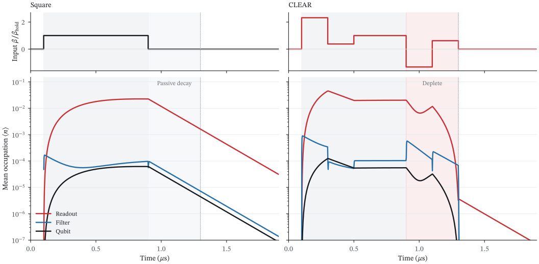
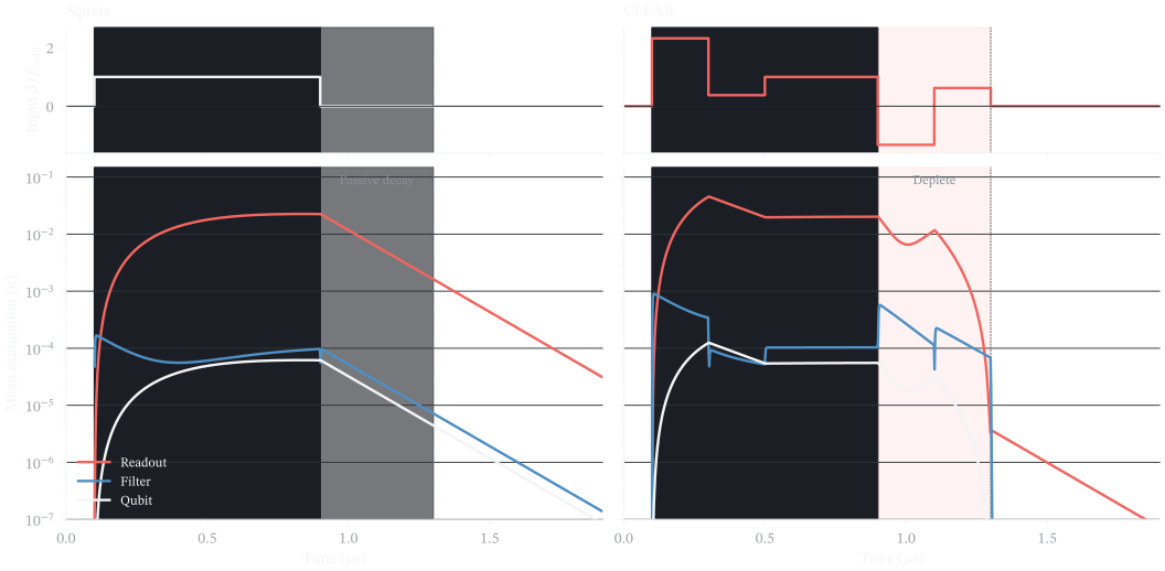
Ground-state preparation; occupations are averaged over 2 ns bins. CLEAR uses extra drive during loading and depletion. Its final segments remove readout photons much faster than waiting over the same 900–1300 ns interval. The small qubit occupation includes hybridization with the resonator. PDF

The IQ paths show how the depletion segments move the coherent readout field back toward zero for both qubit preparations.

Plot the readout IQ trajectories

figure, axes = plt.subplots(1, 2, figsize=(5.6, 3.3), sharex=True, sharey=True, layout='constrained')
readout_end = np.searchsorted(clear_times, 900)
reset_end = np.searchsorted(clear_times, 1300)
for axis, name in zip(axes, ('Square', 'CLEAR')):
    for level, color in ((0, '#246FA8'), (1, '#C92F33')):
        iq = clear_iq[name][level]
        axis.plot(iq[:readout_end+1].real, iq[:readout_end+1].imag, color=color, lw=1.7,
                  label=fr'Prepared $|{level}\rangle$')
        axis.plot(iq[readout_end:reset_end+1].real, iq[readout_end:reset_end+1].imag,
                  color=color, ls='--', lw=1.7)
        axis.plot(iq[readout_end].real, iq[readout_end].imag, 's', color=color, ms=5)
        axis.plot(iq[reset_end].real, iq[reset_end].imag, 'o', mec=color, mfc='white', mew=1.3, ms=7)
    axis.plot(0, 0, '+', color='#16181C', ms=7, mew=1.2)
    axis.set_title(name)
    axis.set_xlabel(r'$\mathrm{Re}\,\alpha_r$')
    axis.set_aspect('equal', adjustable='box')

axes[0].set_ylabel(r'$\mathrm{Im}\,\alpha_r$')

axes[0].legend(fontsize=9, loc='upper left')

figure.savefig("../docs/images/clear_iq.svg")
plt.show()

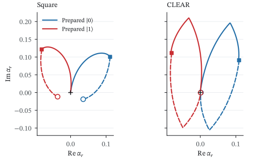
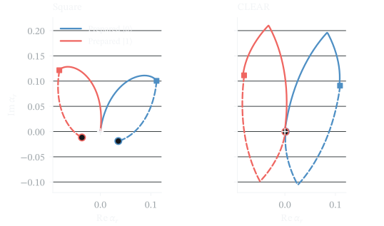
Squares mark 900 ns; open circles mark 1300 ns. Dashed paths cover that interval. CLEAR brings both mean fields close to the origin. These paths show coherent-field cancellation; |⟨aᵣ⟩|² is not the total photon occupation. PDF

Check depletion at the same elapsed time

reset_index = np.searchsorted(clear_times, 1300)
for values in clear_occupations.values():
    assert np.all(np.isfinite(values))
assert clear_occupations["CLEAR"][1, 0, reset_index] < clear_occupations["Square"][1, 0, reset_index] / 100
for level in (0, 1):
    assert clear_dressed.assignment_overlaps[(level, 0, 0)] > 0.99
    assert abs(clear_iq["CLEAR"][level, reset_index])**2 < abs(clear_iq["Square"][level, reset_index])**2 / 100

The excited preparation also keeps its dressed qubit excitation, so zero mean field does not mean a vacuum state. For the signal at the instrument ports, continue with readout and fridge wiring.

To measure a saved state without a simulated readout pulse, continue with qubit readout through the fridge.