Statics and parameter studies

Start from one declared chip. Read dressed quantities and change one parameter, then track an avoided crossing and its state assignments. The final example compares a fluxonium model with published spectroscopy and readout data. This guide does not create a QuantumSequence or evolve a state in time.

quchip uses GHz for frequencies and couplings.

Declare and read a chip

Declare the devices, read their dressed transitions, then vary one bare frequency.

from quchip import Capacitive, Chip, DuffingTransmon, Resonator

q1 = DuffingTransmon(freq=5.30, anharmonicity=-0.65, levels=4, label="q1")
q2 = DuffingTransmon(freq=5.58, anharmonicity=-0.65, levels=4, label="q2")
bus = Resonator(freq=6.55, levels=4, label="bus")
chip = Chip(
    [q1, q2, bus],
    [
        Capacitive(q1, bus, g=0.05),
        Capacitive(q2, bus, g=0.05),
    ],
    frame="rotating",
)

{
    "dressed_f01_ghz": {
        device.label: float(chip.freq(device)) for device in chip.devices
    },
    "static_zz_ghz": float(chip.static_zz(q1, q2)),
}

Output:

{'dressed_f01_ghz': {'q1': 5.297749744925113,
  'q2': 5.577226664394395,
  'bus': 6.55414143998032},
 'static_zz_ghz': 2.2604309073415152e-05}

Change one design parameter

with_params() returns a new chip. Parameter paths come from component labels, so the change remains readable at the call site and the original chip keeps its declaration.

shifted_chip = chip.with_params({"q2.freq": 5.40})

{
    "available_parameters": tuple(chip.parameters),
    "original_q2_freq": chip.parameters["q2.freq"],
    "shifted_q2_freq": shifted_chip.parameters["q2.freq"],
    "shifted_dressed_q2_freq": float(shifted_chip.freq("q2")),
}

Output:

{'available_parameters': ('q1.freq',
  'q1.anharmonicity',
  'q2.freq',
  'q2.anharmonicity',
  'bus.freq',
  'cap_0.g',
  'cap_1.g'),
 'original_q2_freq': 5.58,
 'shifted_q2_freq': 5.4,
 'shifted_dressed_q2_freq': 5.39765272276005}

Resolve the avoided crossing

Two multilevel transmons couple through a detuned bus resonator. Sweeping one bare transmon frequency through the other makes the bare declarations cross. The dressed transitions remain separated by twice the bus-mediated exchange rate.

quchip uses GHz for frequencies. The model below uses the same parameters as the slide and applies RWA() in a rotating frame.

import json

import matplotlib.pyplot as plt
import numpy as np

from quchip import RWA, Capacitive, ChargeDrive, Chip, DuffingTransmon, Resonator, SpectrumSweep, Sweep

q1_frequency = 5.30
q2_frequency0 = 5.58
bus_frequency = 6.55
q2_frequencies = np.linspace(5.255, 5.345, 181)
coupling_strength = 0.050

q1 = DuffingTransmon(
    freq=q1_frequency,
    anharmonicity=-0.65,
    levels=4,
    label="q1",
)
q2 = DuffingTransmon(
    freq=q2_frequency0,
    anharmonicity=-0.65,
    levels=4,
    label="q2",
)
bus = Resonator(freq=bus_frequency, levels=4, label="bus")
chip = Chip(
    [q1, q2, bus],
    couplings=[
        Capacitive(q1, bus, g=coupling_strength, label="q1-bus"),
        Capacitive(q2, bus, g=coupling_strength, label="q2-bus"),
    ],
    frame="rotating",
    approximation=RWA(),
)
q1_line = ChargeDrive(q1, label="q1-charge")
_ = chip.wire(q1_line)

Read the chip’s statics

The declared frequencies are inputs. chip.freq() returns dressed \(0\rightarrow1\) transitions, while chip.static_zz() returns the conditional two-qubit shift for this coupled model.

initial_dressed_frequencies = {
    "q1": float(chip.freq(q1)),
    "q2": float(chip.freq(q2)),
    "bus": float(chip.freq(bus)),
}
initial_static_zz = float(chip.static_zz(q1, q2))
kerr = chip.kerr_matrix()

assert np.isclose(kerr[q1, q1], chip.dressed_anharmonicity(q1))
assert np.isclose(kerr[q1, bus], chip.dispersive_shift(q1, bus))

static_snapshot = {
    "q1_f01_ghz": float(chip.freq(q1)),
    "q1_f12_ghz": float(chip.transition_frequency(q1, 1, 2)),
    "kerr_labels": kerr.labels,
    "kerr_matrix_ghz": np.asarray(kerr.values),
    "q1_drive_matrix_element": complex(
        chip.drive_matrix_elements(q1, drives=[q1_line])[q1_line]
    ),
}

static_snapshot

Output:

{'q1_f01_ghz': 5.297749744925113,
 'q1_f12_ghz': 4.64911449272806,
 'kerr_labels': ('q1', 'q2', 'bus'),
 'kerr_matrix_ghz': array([[-6.48635252e-01,  2.26043091e-05, -1.37823836e-03],
        [ 2.26043091e-05, -6.48041520e-01, -2.06691858e-03],
        [-1.37823836e-03, -2.06691858e-03, -4.50706699e-06]]),
 'q1_drive_matrix_element': -0.9989561107920195j}

kerr_matrix() gathers the dressed anharmonicities on its diagonal and the full-pull cross-Kerr shifts off diagonal, in chip.devices order. The two assertions above check its entries against the scalar APIs.

The resolved Hamiltonian applies the chip’s basis, frame, and approximation strategy through the same public path used for simulation.

chip.hamiltonian()

Output:

\[1\,\hat H_0 + f_{coupling,0}\!\left(t\right)\,\hat H_{coupling,0} + f_{coupling,1}\!\left(t\right)\,\hat H_{coupling,1} + f_{coupling,2}\!\left(t\right)\,\hat H_{coupling,2} + f_{coupling,3}\!\left(t\right)\,\hat H_{coupling,3}\]

chip.resolve().dropped_terms_summary() audits the RWA without reconstructing the Hamiltonian by hand:

rwa_summary = chip.resolve().dropped_terms_summary()
print(rwa_summary)

Output:

4 term(s) dropped:
  [q1-bus] coupling band (Δa=-1, Δb=-1) on q1·bus  (counter-rotating under RWA; amp 0.15 GHz, freq 11.8519 GHz)
  [q1-bus] coupling band (Δa=+1, Δb=+1) on q1·bus  (counter-rotating under RWA; amp 0.15 GHz, freq 11.8519 GHz)
  [q2-bus] coupling band (Δa=-1, Δb=-1) on q2·bus  (counter-rotating under RWA; amp 0.15 GHz, freq 12.1314 GHz)
  [q2-bus] coupling band (Δa=+1, Δb=+1) on q2·bus  (counter-rotating under RWA; amp 0.15 GHz, freq 12.1314 GHz)

Sweep one bare frequency

Sweep names the public parameter path to vary. SpectrumSweep creates an isolated chip at each point, so the original declaration remains unchanged. Setting overlap_threshold=0.0 keeps both intentionally hybridized one-excitation labels available at the centre of the avoided crossing.

frequency_axis = Sweep(q2_frequencies, name="q2.freq")
sweep_result = SpectrumSweep(
    chip,
    [frequency_axis],
    evals_count=4,
    overlap_threshold=0.0,
).run(progress=False)

The two lowest excited eigenvalues are the qubit-like branches throughout this window; the bus-like excitation remains far above them. Subtracting the ground energy at each sweep point gives the two transition frequencies. The public dressed_index() result tells us which branch is more \(q_1\)-like.

ground_energy = sweep_result.eigenvalues[:, 0]
qubit_branches = sweep_result.eigenvalues[:, 1:3] - ground_energy[:, None]
lower_branch = qubit_branches[:, 0]
upper_branch = qubit_branches[:, 1]
splitting = upper_branch - lower_branch
q1_branch = sweep_result.dressed_index(q1=1, q2=0, bus=0).astype(int) - 1

minimum_index = int(np.argmin(splitting))
minimum_splitting = float(splitting[minimum_index])
minimum_frequency = float(q2_frequencies[minimum_index])
inferred_exchange_rate = 0.5 * minimum_splitting
second_order_splitting_scale = 2.0 * coupling_strength**2 / abs(bus_frequency - q1_frequency)
relative_difference_to_second_order = (
    abs(minimum_splitting - second_order_splitting_scale) / minimum_splitting
)

if minimum_index in (0, len(q2_frequencies) - 1):
    raise RuntimeError("The avoided-crossing minimum lies at the sweep boundary.")
if not 4.3e-3 < minimum_splitting < 4.5e-3:
    raise RuntimeError("The resolved splitting does not reproduce the slide-scale exchange rate.")
if len(chip.resolve().dropped_terms) != 4:
    raise RuntimeError("The RWA ledger does not contain the four counter-rotating coupling bands.")
if chip.parameters["q2.freq"] != q2_frequency0:
    raise RuntimeError("SpectrumSweep mutated the original chip.")

Interpret the avoided crossing

The dashed lines are the bare declarations. Red follows the more \(q_1\)-like dressed transition, and black follows the more \(q_2\)-like transition. At the crossing, the branches remain separated by \(2J\approx4.4\) MHz. Second-order dispersive perturbation theory gives \(4.0\) MHz. The resolved spectrum includes the higher-order dressing retained by this truncated model. The lower panel shows why a bare-state label needs care at the crossing: its assignment weight falls to about one half as the two excitations hybridize.

q1_assignment = sweep_result.dressed_index(q1=1, q2=0, bus=0)
q1_label = (1, 0, 0)
q1_label_position = sweep_result.bare_labels.index(q1_label)
q1_assignment_overlap = np.asarray(
    sweep_result.assignment_overlaps[..., q1_label_position]
)

figure, (axis, overlap_axis) = plt.subplots(
    2,
    1,
    figsize=(7.4, 6.2),
    height_ratios=(3.0, 1.0),
    sharex=True,
    layout="constrained",
)

axis.plot(q2_frequencies, q2_frequencies, color="0.78", linestyle="--", linewidth=1.1)
axis.axhline(q1_frequency, color="0.78", linestyle="--", linewidth=1.1, label="bare declarations")
for branch_index in (0, 1):
    q1_like = q1_branch == branch_index
    axis.plot(
        q2_frequencies,
        np.where(q1_like, qubit_branches[:, branch_index], np.nan),
        color="#C92F33",
        linewidth=2.3,
        label="$q_1$-like" if branch_index == 0 else None,
    )
    axis.plot(
        q2_frequencies,
        np.where(~q1_like, qubit_branches[:, branch_index], np.nan),
        color="#16181C",
        linewidth=2.3,
        label="$q_2$-like" if branch_index == 0 else None,
    )
axis.annotate(
    f"$2J$ = {1.0e3 * minimum_splitting:.1f} MHz",
    xy=(minimum_frequency, 0.5 * (lower_branch[minimum_index] + upper_branch[minimum_index])),
    xytext=(5.327, 5.270),
    arrowprops={"arrowstyle": "-", "color": "0.35"},
    fontsize=10,
)
axis.set(
    ylabel="Transition frequency (GHz)",
    xlim=(q2_frequencies[0], q2_frequencies[-1]),
)
axis.legend(frameon=False, ncols=2, loc="upper left")

overlap_axis.plot(
    q2_frequencies,
    q1_assignment_overlap,
    color="#246FA8",
    linewidth=2.0,
)
overlap_axis.axhline(0.5, color="0.72", linestyle="--", linewidth=1.0)
overlap_axis.set(
    xlabel="Bare q2 frequency (GHz)",
    ylabel=r"$q_1$ assignment",
    ylim=(0.45, 1.02),
)

figure_path = "../docs/images/resolve_and_sweep.png"
figure.savefig(figure_path, dpi=180)
plt.show()

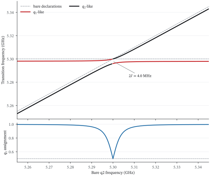
The bare declarations cross while the dressed transitions retain a finite splitting. The assignment weight exposes the hybridized region directly.

The receipt records the exchange inferred from the avoided crossing, the second-order scale, the approximation audit, and whether the original chip kept its declared q2 frequency.

statics_receipt = {
    "approximation": chip.settings["approximation"],
    "dressed_frequencies_ghz": initial_dressed_frequencies,
    "dropped_rwa_terms": len(chip.resolve().dropped_terms),
    "figure": figure_path,
    "full_dimension": int(np.prod(chip.dims)),
    "inferred_exchange_rate_mhz": 1.0e3 * inferred_exchange_rate,
    "minimum_at_bare_q2_ghz": minimum_frequency,
    "minimum_splitting_mhz": 1.0e3 * minimum_splitting,
    "original_chip_unchanged": bool(chip.parameters["q2.freq"] == q2_frequency0),
    "relative_difference_to_second_order": relative_difference_to_second_order,
    "second_order_splitting_scale_mhz": 1.0e3 * second_order_splitting_scale,
    "static_zz_khz": 1.0e6 * initial_static_zz,
    "sweep_points": len(q2_frequencies),
}

print(f"RESULT statics={json.dumps(statics_receipt, sort_keys=True, separators=(',', ':'))}")

Output:

RESULT statics={"approximation":"RWA","dressed_frequencies_ghz":{"bus":6.55414143998032,"q1":5.297749744925113,"q2":5.577226664394395},"dropped_rwa_terms":4,"figure":"../docs/images/resolve_and_sweep.png","full_dimension":64,"inferred_exchange_rate_mhz":2.204908100780223,"minimum_at_bare_q2_ghz":5.3,"minimum_splitting_mhz":4.409816201560446,"original_chip_unchanged":true,"relative_difference_to_second_order":0.09293271710857891,"second_order_splitting_scale_mhz":4.000000000000001,"static_zz_khz":22.604309073415152,"sweep_points":181}

Independent and linked parameter studies

Sweep.expand() shows the parameter dictionaries before any calculation runs. Independent axes form a Cartesian grid. Sweep.zip() pairs values when the parameters must move together.

frequency_values = Sweep([5.28, 5.30, 5.32], name="q2.freq")
coupling_values = Sweep([0.045, 0.050], name="q1-bus.g")
independent_points = Sweep.expand([frequency_values, coupling_values])

linked_points = Sweep.expand(
    [
        Sweep.zip(
            Sweep([5.28, 5.30, 5.32], name="q2.freq"),
            Sweep([0.045, 0.050, 0.055], name="q1-bus.g"),
        )
    ]
)

{
    "independent_point_count": len(independent_points),
    "first_independent_point": independent_points[0],
    "linked_point_count": len(linked_points),
    "last_linked_point": linked_points[-1],
}

Output:

{'independent_point_count': 6,
 'first_independent_point': {'q2.freq': np.float64(5.28),
  'q1-bus.g': np.float64(0.045)},
 'linked_point_count': 3,
 'last_linked_point': {'q2.freq': np.float64(5.32),
  'q1-bus.g': np.float64(0.055)}}

Pass either axis list to SpectrumSweep when every point needs a dressed spectrum. Use with_params() directly when only a few points or a custom observable are needed.

Check labels before interpreting branches

Near an avoided crossing, a dressed eigenstate can be shared between several bare product states. dressed_index() tracks the assigned branch across the sweep, while assignment_overlaps records how confident that assignment is. For one chip, state_components() exposes the largest bare-basis weights.

q1_components = chip.state_components({q1: 1}, n_components=4)

{
    "tracked_grid_shape": q1_assignment.shape,
    "lowest_q1_assignment_overlap": float(np.nanmin(q1_assignment_overlap)),
    "q1_like_state_components": q1_components,
}

Output:

{'tracked_grid_shape': (181,),
 'lowest_q1_assignment_overlap': 0.49837736639905067,
 'q1_like_state_components': {(1, 0, 0): 0.9982630319848723,
  (0, 0, 1): 0.0016179267171988069,
  (0, 1, 0): 6.181316921618551e-05,
  (2, 0, 1): 3.98212745963501e-05}}

Do not force a bare label through a strongly hybridized region without reading the overlaps. The value near 0.5 occurs at the centre of this crossing, where the two bare qubit excitations share the dressed branches. Setting a lower overlap_threshold keeps a branch available; it does not make the bare-state description more accurate.

Check numerical resolution

The sweep grid locates the minimum; device levels control Hilbert-space truncation. They are separate convergence questions. Here the 181-point grid and its every-other-point subset agree because both contain the symmetry point.

fine_minimum = float(np.min(splitting))
coarse_minimum = float(np.min(splitting[::2]))

{
    "fine_grid_points": len(splitting),
    "coarse_grid_points": len(splitting[::2]),
    "minimum_difference_hz": 1.0e9 * abs(fine_minimum - coarse_minimum),
}

Output:

{'fine_grid_points': 181,
 'coarse_grid_points': 91,
 'minimum_difference_hz': 0.0}

For a truncation check, rebuild the devices with one extra level and compare the observable you intend to report. A stable transition does not guarantee a stable matrix element or dispersive shift, so check the actual output.

Paper example: experimental fluxonium spectroscopy

Stefanski et al. measured a fluxonium and its readout resonator while sweeping external flux. Their paper, Improved fluxonium readout through dynamic flux pulsing, reports the fitted circuit parameters and the operating points used for readout. The authors also publish their analysis and modelling code and the measurement archive.

We first reproduce the qubit spectrum with one Fluxonium. The readout resonator is added afterward.

Load the published measurements

The repository supplies extracted frequencies, so no image digitization is needed. processed_data_fx8.csv stores the measured qubit frequency and the five parameters fitted by the authors. res_fit_results.csv stores the two state-dependent resonator frequencies and their half-difference \(\chi=(f_{r,1}-f_{r,0})/2\).

import csv
import io
from urllib.request import urlopen

from quchip import CouplingModel, Fluxonium, Scalar, parameter

paper_data_root = (
    "https://raw.githubusercontent.com/AndersenQubitLab/"
    "FPA-RO-experimental/57dc268dd048d1372db082c3ddd97a04871580bf"
)


def published_rows(filename):
    url = f"{paper_data_root}/{filename}"
    with urlopen(url) as response:  # noqa: S310 - fixed public research archive
        return list(csv.DictReader(io.StringIO(response.read().decode("utf-8"))))


spectrum_rows = published_rows("processed_data_fx8.csv")
readout_rows = published_rows("res_fit_results.csv")

fitted_values = np.asarray(
    [float(spectrum_rows[index]["energy_params"]) for index in range(5)]
)
resonator_frequency, readout_coupling, paper_E_J, paper_E_C, paper_E_L = fitted_values

paper_parameters = {
    "E_J_ghz": paper_E_J,
    "E_C_ghz": paper_E_C,
    "E_L_ghz": paper_E_L,
    "resonator_frequency_ghz": resonator_frequency,
    "readout_coupling_ghz": readout_coupling,
}
paper_parameters

Output:

{'E_J_ghz': np.float64(3.8217399868188027),
 'E_C_ghz': np.float64(0.8652719648666846),
 'E_L_ghz': np.float64(0.8215798519627777),
 'resonator_frequency_ghz': np.float64(5.175140901166961),
 'readout_coupling_ghz': np.float64(0.037156311892102264)}

Reproduce the qubit spectrum

Figure 2 of the paper covers \(0.5\leq\Phi_{\mathrm{ext}}/\Phi_0\leq0.85\). The model curve uses 351 evenly spaced flux values, more than twice the measurement density. Residuals are evaluated by interpolating that independent curve at the measured coordinates. quchip receives the authors’ fitted energies unchanged.

paper_flux_all = np.asarray(
    [float(row["phi_ext_qubit"]) for row in spectrum_rows if row["phi_ext_qubit"]]
)
measured_f01_all = np.asarray(
    [float(row["qubit_freq"]) for row in spectrum_rows if row["qubit_freq"]]
)
figure_2_window = paper_flux_all <= 0.85
paper_flux = paper_flux_all[figure_2_window]
measured_f01 = measured_f01_all[figure_2_window]


def isolated_f01(phi_ext):
    q = Fluxonium(
        E_C=paper_E_C,
        E_J=paper_E_J,
        E_L=paper_E_L,
        phi_ext=phi_ext,
        levels=4,
        num_basis=300,
        phi_max=5.0 * np.pi,
        basis="eigen",
        label="q",
    )
    return float(q.freq)


paper_model_flux = np.linspace(0.5, 0.85, 351)
predicted_f01_grid = np.asarray([isolated_f01(phi) for phi in paper_model_flux])
predicted_f01_at_data = np.interp(paper_flux, paper_model_flux, predicted_f01_grid)
f01_residual_mhz = 1.0e3 * (predicted_f01_at_data - measured_f01)

paper_spectrum_figure, (spectrum_axis, residual_axis) = plt.subplots(
    2,
    1,
    figsize=(7.4, 6.0),
    sharex=True,
    gridspec_kw={"height_ratios": [2.3, 1.0]},
    layout="constrained",
)
spectrum_axis.scatter(
    paper_flux,
    measured_f01,
    s=15,
    color="#262626",
    alpha=0.7,
    label="experiment",
)
spectrum_axis.plot(
    paper_model_flux,
    predicted_f01_grid,
    color="#C92F33",
    linewidth=2.2,
    label="quchip",
)
spectrum_axis.set_ylabel(r"$f_{01}$ (GHz)")
spectrum_axis.legend(frameon=False)
spectrum_axis.grid(color="0.88", linewidth=0.7)

residual_axis.axhline(0.0, color="0.45", linewidth=1.0)
residual_axis.scatter(paper_flux, f01_residual_mhz, s=14, color="#246FA8", alpha=0.78)
residual_axis.set(
    xlabel=r"External flux $\Phi_{\mathrm{ext}}/\Phi_0$",
    ylabel="model - data\n(MHz)",
)
residual_axis.grid(color="0.88", linewidth=0.7)

paper_spectrum_path = "../docs/images/stefanski_fluxonium_spectrum.png"
paper_spectrum_figure.savefig(paper_spectrum_path, dpi=180)
plt.show()

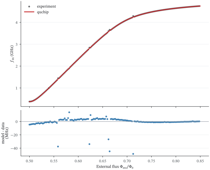
The authors’ fitted fluxonium energies reproduce the measured frequency curve. Every extracted point in the paper’s Figure 2 window is shown.

spectrum_check = {
    "measurement_points": len(measured_f01),
    "median_absolute_error_mhz": float(np.median(np.abs(f01_residual_mhz))),
    "p95_absolute_error_mhz": float(np.quantile(np.abs(f01_residual_mhz), 0.95)),
    "rmse_mhz": float(np.sqrt(np.mean(f01_residual_mhz**2))),
    "points_above_10_mhz": int(np.count_nonzero(np.abs(f01_residual_mhz) > 10.0)),
}
spectrum_check

Output:

{'measurement_points': 153,
 'median_absolute_error_mhz': 1.5923938298039175,
 'p95_absolute_error_mhz': 6.076768528398682,
 'rmse_mhz': 7.573880277392135,
 'points_above_10_mhz': 6}

The six residuals above 10 MHz remain in the plot and in the RMSE. The median and 95th percentile describe the rest of the curve without deleting those points.

Add the readout resonator

The released model couples a resonator to the fluxonium oscillator coordinate \(c\) through \(g(ca^\dagger+c^\dagger a)\). CouplingModel is quchip’s public extension point for declaring that interaction without changing the device models.

class FluxoniumReadoutCoupling(CouplingModel):
    """Exchange interaction used in the authors' released readout model."""

    g: Scalar = parameter(unit="GHz")
    oscillator_length: Scalar = parameter(positive=True)

    def interaction(self, q, r, p):
        scale = np.sqrt(2.0)
        lowering = q.phi * (1.0 / (p.oscillator_length * scale)) + (
            1j * p.oscillator_length / scale
        ) * q.charge
        raising = q.phi * (1.0 / (p.oscillator_length * scale)) - (
            1j * p.oscillator_length / scale
        ) * q.charge
        return p.g * (lowering * r.adag + raising * r.a)


paper_q = Fluxonium(
    E_C=paper_E_C,
    E_J=paper_E_J,
    E_L=paper_E_L,
    phi_ext=0.5,
    levels=10,
    num_basis=300,
    phi_max=5.0 * np.pi,
    basis="eigen",
    label="q",
)
paper_readout = Resonator(freq=resonator_frequency, levels=3, label="readout")
paper_edge = FluxoniumReadoutCoupling(
    paper_q,
    paper_readout,
    g=readout_coupling,
    oscillator_length=(8.0 * paper_E_C / paper_E_L) ** 0.25,
    label="q-readout",
)
paper_chip = Chip(
    [paper_q, paper_readout],
    [paper_edge],
    basis="eigen",
    frame="lab",
)

chip.freq("readout") is the resonator transition with the qubit in \(|0\rangle\). chip.dispersive_shift() returns the full state-dependent pull, so the paper’s \(\chi\) is half of it.

readout_rows = [row for row in readout_rows if row["phi_ext_disshift"]]
readout_flux_all = np.asarray([float(row["phi_ext_disshift"]) for row in readout_rows])
measured_fr0_all = np.asarray([float(row["fr_q0"]) for row in readout_rows])
measured_fr1_all = np.asarray([float(row["fr_q1"]) for row in readout_rows])
measured_chi_all = np.asarray([float(row["chi"]) for row in readout_rows])

readout_window = readout_flux_all <= 0.85
readout_flux = readout_flux_all[readout_window]
measured_fr0 = measured_fr0_all[readout_window]
measured_fr1 = measured_fr1_all[readout_window]
measured_chi_mhz = measured_chi_all[readout_window]


def readout_observables(phi_ext):
    point = paper_chip.with_params({"q.phi_ext": phi_ext})
    fr0 = float(point.freq("readout"))
    full_pull = float(point.dispersive_shift("q", "readout"))
    return fr0, fr0 + full_pull, 500.0 * full_pull


readout_model_flux = np.linspace(0.5, 0.85, 351)
predicted_readout_grid = np.asarray(
    [readout_observables(phi) for phi in readout_model_flux]
)
predicted_fr0_grid = predicted_readout_grid[:, 0]
predicted_fr1_grid = predicted_readout_grid[:, 1]
predicted_chi_grid_mhz = predicted_readout_grid[:, 2]

predicted_fr0_at_data = np.interp(readout_flux, readout_model_flux, predicted_fr0_grid)
predicted_fr1_at_data = np.interp(readout_flux, readout_model_flux, predicted_fr1_grid)
predicted_chi_at_data_mhz = np.interp(
    readout_flux,
    readout_model_flux,
    predicted_chi_grid_mhz,
)

readout_figure, (frequency_axis, chi_axis) = plt.subplots(
    2,
    1,
    figsize=(7.4, 6.0),
    sharex=True,
    layout="constrained",
)
frequency_axis.scatter(readout_flux, measured_fr0, s=12, color="#C92F33", alpha=0.6)
frequency_axis.scatter(readout_flux, measured_fr1, s=12, color="#246FA8", alpha=0.6)
frequency_axis.plot(
    readout_model_flux,
    predicted_fr0_grid,
    color="#C92F33",
    label=r"$q=|0\rangle$",
)
frequency_axis.plot(
    readout_model_flux,
    predicted_fr1_grid,
    color="#246FA8",
    label=r"$q=|1\rangle$",
)
frequency_axis.set_ylabel("Readout frequency (GHz)")
frequency_axis.legend(frameon=False, ncols=2)
frequency_axis.grid(color="0.88", linewidth=0.7)

chi_axis.scatter(
    readout_flux,
    measured_chi_mhz,
    s=13,
    color="#262626",
    alpha=0.62,
    label="experiment",
)
chi_axis.plot(
    readout_model_flux,
    predicted_chi_grid_mhz,
    color="#246FA8",
    linewidth=2.0,
    label="quchip",
)
chi_axis.set(
    xlabel=r"External flux $\Phi_{\mathrm{ext}}/\Phi_0$",
    ylabel=r"$\chi$ (MHz)",
)
chi_axis.legend(frameon=False)
chi_axis.grid(color="0.88", linewidth=0.7)

paper_readout_path = "../docs/images/stefanski_fluxonium_readout.png"
readout_figure.savefig(paper_readout_path, dpi=180)
plt.show()

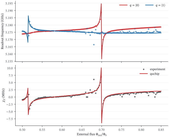
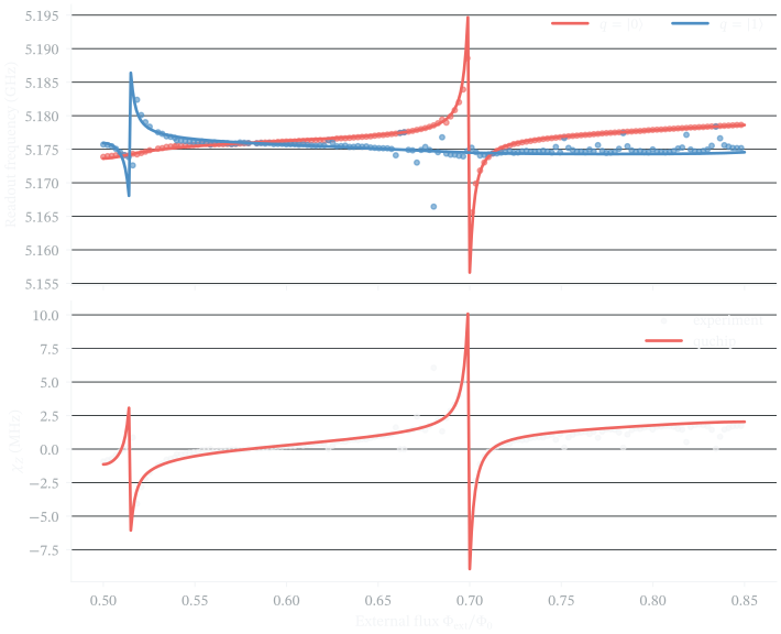
The same chip reproduces the state-dependent readout frequencies and the higher-level resonances in the dispersive shift.

The paper operates at the sweet spot for idle and control, then pulses to \(\Phi_{\mathrm{ext}}/\Phi_0=0.6567\) during readout. These two points give a compact numerical check against the values quoted in the text.

sweet_spot = readout_observables(0.5)
flux_pulsed = readout_observables(0.6567)

operating_points = {
    "sweet_spot": {
        "paper_f01_ghz": 0.377,
        "quchip_f01_ghz": isolated_f01(0.5),
        "paper_fr0_ghz": 5.1739,
        "quchip_fr0_ghz": sweet_spot[0],
        "paper_chi_mhz": 0.92,
        "quchip_chi_mhz": sweet_spot[2],
    },
    "flux_pulsed_readout": {
        "paper_flux": 0.6567,
        "paper_f01_ghz": 3.47,
        "quchip_f01_ghz": isolated_f01(0.6567),
        "paper_chi_mhz": -1.09,
        "quchip_chi_mhz": flux_pulsed[2],
    },
}
operating_points

Output:

{'sweet_spot': {'paper_f01_ghz': 0.377,
  'quchip_f01_ghz': 0.37229583974984704,
  'paper_fr0_ghz': 5.1739,
  'quchip_fr0_ghz': 5.173631975636763,
  'paper_chi_mhz': 0.92,
  'quchip_chi_mhz': 1.1418029950291952},
 'flux_pulsed_readout': {'paper_flux': 0.6567,
  'paper_f01_ghz': 3.47,
  'quchip_f01_ghz': 3.4802282134309697,
  'paper_chi_mhz': -1.09,
  'quchip_chi_mhz': -1.1351841383457906}}

resonator_residual_mhz = 1.0e3 * np.concatenate(
    [predicted_fr0_at_data - measured_fr0, predicted_fr1_at_data - measured_fr1]
)
chi_residual_mhz = predicted_chi_at_data_mhz - measured_chi_mhz

paper_receipt = {
    "chi_median_absolute_error_mhz": float(np.median(np.abs(chi_residual_mhz))),
    "chi_rmse_mhz": float(np.sqrt(np.mean(chi_residual_mhz**2))),
    "readout_frequency_rmse_mhz": float(
        np.sqrt(np.mean(resonator_residual_mhz**2))
    ),
    "readout_points": len(readout_flux),
    "readout_model_points": len(readout_model_flux),
    "spectrum_median_absolute_error_mhz": spectrum_check["median_absolute_error_mhz"],
    "spectrum_p95_absolute_error_mhz": spectrum_check["p95_absolute_error_mhz"],
    "spectrum_points": len(paper_flux),
    "spectrum_model_points": len(paper_model_flux),
}

print(
    "RESULT paper_statics="
    + json.dumps(paper_receipt, sort_keys=True, separators=(",", ":"))
)

Output:

RESULT paper_statics={"chi_median_absolute_error_mhz":0.1767470986042987,"chi_rmse_mhz":0.7651558998064468,"readout_frequency_rmse_mhz":1.0847642735011658,"readout_model_points":351,"readout_points":151,"spectrum_median_absolute_error_mhz":1.5923938298039175,"spectrum_model_points":351,"spectrum_p95_absolute_error_mhz":6.076768528398682,"spectrum_points":153}

The paper’s authors fitted the circuit parameters to these measurements. Treat this result as a cross-implementation check of their static model. A fabrication-level prediction would require independent circuit parameters.

Choose the static observable

Use freq() and transition_frequency() for dressed transitions, kerr_matrix() for several dressed self-Kerr and cross-Kerr coefficients, dressed_anharmonicity() for one level curvature, dispersive_shift() or static_zz() for one conditional shift, drive_matrix_elements() for control strengths, and state_components() for hybridization. SpectrumSweep keeps the eigenvalues, assignments, overlaps, and grid shape together.

Change either bus coupling and rerun the sweep to see how the inferred exchange changes. Moving the bus closer tests where the second-order dispersive scale stops tracking the resolved avoided crossing.