

What happens during a qubit measurement?
A qubit starts in \(|+\rangle=(|0\rangle+|1\rangle)/\sqrt{2}\). When we monitor \(\sigma_z\), some trajectories go quickly toward a pole, while others wander or reverse direction before they settle. Generate these individual histories and the ensemble density from the same dispersive-readout model.
Murch et al. (2013) tracked conditional superconducting-qubit states and checked them with tomography on repeated preparations. Here we simulate ideal detection and no intrinsic qubit decay. The figures show those measurement dynamics. They do not fit the experiment’s finite-efficiency data or perform an experimental tomography validation.
Set the measurement strength from the resonator
The resonator has a 20 MHz linewidth and a full conditional frequency pull of \(-4\) MHz. Drive halfway between its two conditional resonances, then compare the steady fields for the qubit in \(|0\rangle\) and \(|1\rangle\). Apply a 400 ns square readout pulse to the coupled qubit and resonator, once from each qubit basis state. The final cavity fields set the measurement rate.
import numpy as np
from quchip import (
    RWA, ChargeDrive, Chip, CrossKerr, Qubit, QuantumSequence, Resonator, Square,
)

amplitude = 0.008                     # charge-drive amplitude, GHz
kappa = 2 * np.pi * 0.020             # resonator linewidth, 1/ns
q = Qubit(freq=5.0, label="q")
r = Resonator(freq=6.0, levels=12, T1=1 / kappa, label="r")
readout = Chip(
    [q, r], couplings=[CrossKerr(q, r, chi=-0.004, label="qr")],
    frame={"q": 5.0, "r": 5.998}, approximation=RWA(),
)

drive = ChargeDrive(r, label="readout")
_ = readout.wire(drive)
sequence = QuantumSequence(readout)
_ = sequence.schedule(
    drive, envelope=Square(duration=400.0, amplitude=amplitude), freq=5.998,
)

branches = sequence.simulate_batch(
    sequence.vary("initial_state", [{"q": 0, "r": 0}, {"q": 1, "r": 0}]),
    tlist=np.arange(401.0), e_ops=readout.e_ops(r=["a", "n"]),
    states="none", progress=False,
)

alpha = np.array([branch.expect(r, 0)[-1] for branch in branches])
nbar = float(branches[1].expect(r, 1)[-1].real)
gamma = float(kappa * abs(alpha[0] - alpha[1]) ** 2 / 2)
print(f"Measurement dephasing: {gamma:.8f} /ns; steady photons: {nbar:.6f}")
Output:
Measurement dephasing: 0.00148714 /ns; steady photons: 0.153846
We use the steady-field reduction \(\Gamma_m=\kappa|\alpha_0-\alpha_1|^2/2\),
which \(L=\sqrt{\Gamma_m/2}\,\sigma_z\) represents. Then
\(\mathcal D[L]\rho=(\Gamma_m/2)(\sigma_z\rho\sigma_z-\rho)\), and the
unconditional coherence decays as \(e^{-\Gamma_m t}\). Here gamma means
\(\Gamma_m\), in \(\mathrm{ns}^{-1}\). The cavity settles on a scale
\(2/\kappa\approx16\) ns, much shorter than \(1/\Gamma_m\). The reduced model starts
with the field already settled and tracks out the deterministic Stark rotation,
so it omits the initial cavity transient.
Monitor the qubit
Give the qubit its transition frequency and set the chip to its rotating frame. This
frame removes free precession, and only the measurement backaction stays. T1=None omits
relaxation. T2=1/gamma represents the measurement-induced dephasing, with no additional
unobserved dephasing. The effective frequency includes the steady Stark shift.
The standard channel is \(L=\sqrt{2\Gamma_m}\,n\), with \(n=(I-\sigma_z)/2\). Its dissipator equals the Pauli form above. A homodyne phase of \(\pi\) matches the Pauli trajectory’s noise-sign convention, and the identity offset only changes the record’s baseline. We prepare the bare \(|+\rangle\) because the plotted axes use that Pauli basis.
from quchip import with_monitoring

meter = Qubit(freq=5.0, T1=None, T2=1 / gamma, label="q")
chip = Chip([meter], backend="qutip", frame="rotating")

plus = (chip.bare_state({meter: 0}) + chip.bare_state({meter: 1})) / np.sqrt(2)
t = np.arange(0.0, 1000.0 + 5.0, 5.0)  # saved samples in ns
shots, seed = 3000, 11

problem = QuantumSequence(chip).build_problem(
    t, initial_state=plus, solver="smesolve", states="none",
    e_ops=chip.e_ops(q=[meter.sigma_x, meter.sigma_y, meter.sigma_z]),
    run_args={"ntraj": shots, "seeds": seed},
    options={"method": "platen", "dt": 0.05, "map": "loky", "num_cpus": 4,
             "keep_runs_results": True, "progress_bar": ""},
)

channel = problem.engine_result.slh.channels[0]
result = chip.solve(with_monitoring(problem, {channel.key: 1.0}, phases={channel.key: np.pi}))

bloch = np.empty((shots, len(t), 3))
for i in range(shots):
    trajectory = result.run(i)
    bloch[i] = np.column_stack([trajectory.expect(meter, k).real for k in range(3)])

np.savez_compressed(
    "paths-plus-z.npz", bloch=bloch.astype(np.float32), t=t,
    gamma=gamma, nbar=nbar, amp=amplitude,
)

print(f"Bloch data: {bloch.shape}; final |z| > 0.95: {np.mean(abs(bloch[:, -1, 2]) > 0.95):.3f}")
Output:
Bloch data: (3000, 201, 3); final |z| > 0.95: 0.748
paths-plus-z.npz saves the array with axes (shot, saved time, x/y/z). The file does not keep the
states, because these three observables contain the qubit information used here. dt=0.05 ns sets
the native integration step, and the 5 ns save interval only sets the plot sampling. QuTiP runs the
seeded trajectories across four worker processes, and the loop above only extracts their
observables. The 3,000-shot ensemble includes the four histories shown below.
Compare individual histories
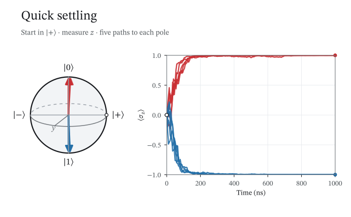
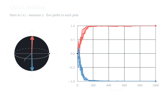
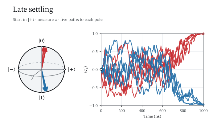
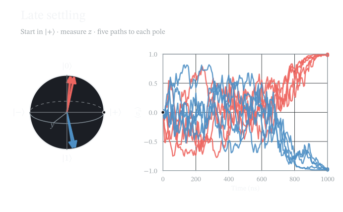
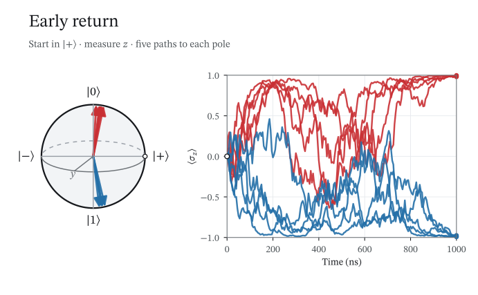
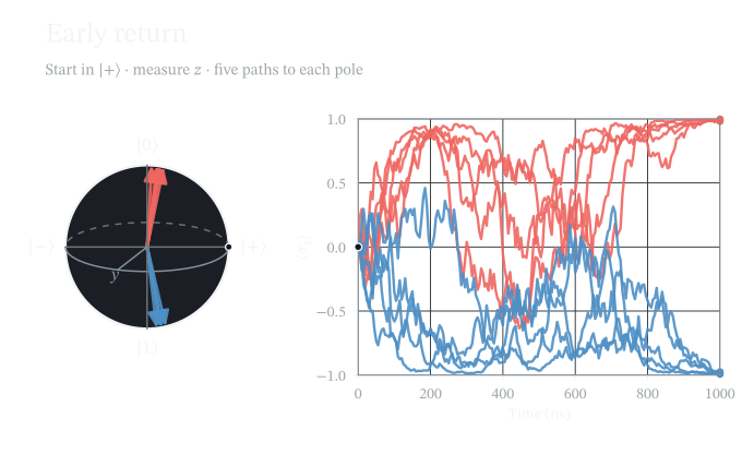
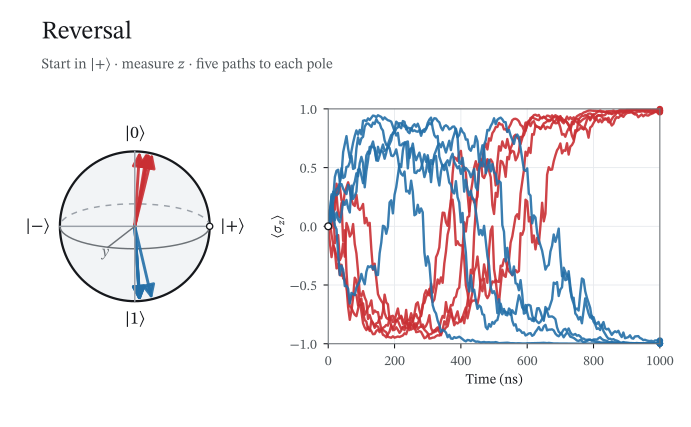
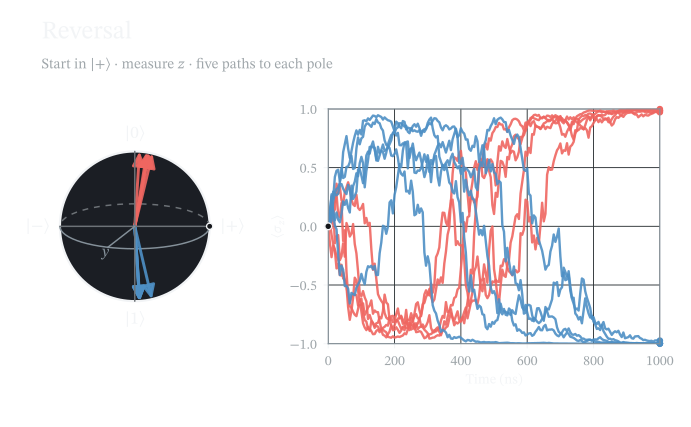
Each video below selects five paths that end near each pole. The selections show different histories in the same ensemble, not disjoint classes or estimates of their prevalence.
“Early return” means that a path approached its eventual pole, then moved away. “Reversal” means that the path first approached the opposite pole. We apply no external kick or relaxation. A state near an eigenstate can reverse, but an exact \(\sigma_z\) eigenstate is stationary under this measurement.
Select and plot the histories
import shutil
import matplotlib.pyplot as plt
from matplotlib.patches import Arc, Circle, FancyArrowPatch

plt.style.use("../docs/_static/quchip.mplstyle")
plt.rcParams["text.usetex"] = bool(shutil.which("latex"))

z = bloch[:, :, 2]
selected = {}
for kind in ("Quick settling", "Late settling", "Early return", "Reversal"):
    selected[kind] = []

    for sign in (1, -1):
        toward = sign * z
        candidates = np.flatnonzero(toward[:, -1] > 0.97)

        if kind == "Quick settling":
            last_outside = np.max(np.where(toward <= 0.95, np.arange(len(t)), -1), axis=1)
            score = -t[np.minimum(last_outside + 1, len(t) - 1)]
        elif kind == "Reversal":
            candidates = candidates[toward[candidates].min(axis=1) < -0.9]
            score = (-toward).max(axis=1)
        else:
            after = t >= (400.0 if kind == "Early return" else 250.0)
            if kind == "Early return":
                early = np.any(toward[:, t <= 400.0] > 0.9, axis=1)
                returned = toward[:, after].min(axis=1) < 0.5
                candidates = candidates[early[candidates] & returned[candidates]]
            score = abs(np.diff(toward[:, after], axis=1)).sum(axis=1) + 4 * (1 - toward[:, after]).mean(axis=1)

        if len(candidates) < 5:
            raise ValueError(f"Too few {kind.lower()} paths toward pole {sign}; increase shots.")

        selected[kind].extend(candidates[np.argsort(-score[candidates])[:5]])

history_figures = {}
for kind, indices in selected.items():
    name = kind.lower().replace(" ", "_")
    fig = plt.figure(figsize=(7.2, 4.45))
    fig.text(0.06, 0.91, kind, fontsize=19)
    fig.text(0.06, 0.84, r"Start in $|+\rangle$ · measure $z$ · five paths to each pole",
             fontsize=11, color="#50565A")

    sphere = fig.add_axes((0.027, 0.198, 0.336, 0.544))
    sphere.set(xlim=(-1.55, 1.55), ylim=(-1.55, 1.55), aspect="equal")
    sphere.axis("off")
    sphere.add_patch(Circle((0, 0), 1, facecolor="#F2F4F6", edgecolor="#16181C", lw=1.7))
    sphere.add_patch(Arc((0, 0), 2, 0.6, theta1=0, theta2=180,
                         color="#9AA0A8", lw=1.1, linestyle=(0, (4, 4))))
    sphere.add_patch(Arc((0, 0), 2, 0.6, theta1=180, theta2=360, color="#6D7277", lw=1.1))
    sphere.plot([-1, 1], [0, 0], color="#9AA0A8", lw=1.1)
    sphere.plot([0, 0], [-1, 1], color="#9AA0A8", lw=1.1)
    sphere.plot([0, -0.36], [0, -0.28], color="#6D7277", lw=1.1)
    sphere.text(-0.45, -0.4, "$y$", color="#6D7277", fontsize=12)

    for x, y, label in ((0, 1.24, r"$|0\rangle$"), (0, -1.24, r"$|1\rangle$"),
                         (1.3, 0, r"$|+\rangle$"), (-1.3, 0, r"$|-\rangle$")):
        sphere.text(x, y, label, ha="center", va="center", fontsize=13)
    sphere.scatter([1], [0], s=22, facecolor="white", edgecolor="#16181C", zorder=20)

    trace = fig.add_axes((0.475, 0.195, 0.48, 0.55))
    trace.set(xlim=(0, t[-1]), ylim=(-1, 1), yticks=(-1, -0.5, 0, 0.5, 1),
              xticks=np.arange(0, 1001, 200), xlabel="Time (ns)", ylabel=r"$\langle\sigma_z\rangle$")
    trace.grid(True)
    for spine in trace.spines.values():
        spine.set_visible(True)
        spine.set_color("#6D7277")

    artists = []
    for i in indices:
        color = "#C92F33" if z[i, -1] > 0 else "#246FA8"
        arrow = FancyArrowPatch((0, 0), bloch[i, -1, [0, 2]],
                                arrowstyle="-|>,head_length=8.4,head_width=3.9",
                                mutation_scale=1, lw=2.2, color=color, alpha=0.9,
                                shrinkA=0, shrinkB=0, capstyle="round", joinstyle="round")
        sphere.add_patch(arrow)
        line, = trace.plot(t, z[i], color=color, lw=1.8, alpha=0.9)
        dot, = trace.plot(t[-1], z[i, -1], "o", color=color, ms=4, clip_on=False)
        artists.append((i, arrow, line, dot))

    trace.scatter([0], [0], s=26, facecolor="white", edgecolor="#16181C", zorder=20, clip_on=False)
    cursor = trace.axvline(t[-1], color="#9AA0A8", lw=1.1, ls=(0, (4, 4)), visible=False)
    history_figures[name] = (fig, artists, cursor)
    fig.savefig(f"../docs/images/measurement_{name}.svg")
    plt.show()
All paths start at \(+x\). Red and blue show the final pole, even before the outcome becomes apparent. The Bloch vectors and moving dots follow the current time, and each trace keeps its history.
Map the ensemble and a selected endpoint
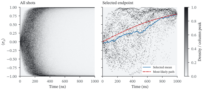
Weber et al. (2014) studied density maps and most-likely paths with both initial and final states specified. For their no-drive case and ideal efficiency, the analytic path from \(z(0)=0\) to \(z(T)=z_f\) is \(z_\mathrm{opt}(t)=\tanh[(t/T)\operatorname{arctanh}(z_f)]\) and \(x_\mathrm{opt}(t)=\sqrt{1-z_\mathrm{opt}(t)^2}\). The paper’s measurement time is \(\tau=1/(2\Gamma_m)\) in our convention.
Select \(z(1000\,\mathrm{ns})=0.8\pm0.03\) from the existing ensemble. The dashed curve is the analytic most-likely path. The solid curve is the selected paths’ mean, which is a different statistic. This no-drive result needs no optimizer or additional solve.
target, window = 0.8, 0.03
conditioned = abs(z[:, -1] - target) < window
optimal = np.tanh(t / t[-1] * np.arctanh(target))
print(f"Endpoint-selected shots: {conditioned.sum()} of {shots}")
Output:
Endpoint-selected shots: 33 of 3000
Plot the two density maps
from matplotlib.colors import LinearSegmentedColormap

edges = np.linspace(-1, 1, 161)
cmap = LinearSegmentedColormap.from_list("measurement", ["#F2F4F6", "#16181C"])
density_images = []

density_fig, axes = plt.subplots(1, 2, figsize=(7.2, 3.2), sharey=True, layout="constrained")
for axis, paths, title in zip(axes, (z, z[conditioned]), ("All shots", "Selected endpoint")):
    counts = np.stack([np.histogram(paths[:, j], bins=edges)[0] for j in range(len(t))], axis=1)
    density = counts.astype(float)
    density /= density.max(axis=0, keepdims=True)
    image = axis.imshow(density, origin="lower", aspect="auto", cmap=cmap, vmin=0, vmax=1,
                        extent=(-2.5, t[-1] + 2.5, -1, 1), interpolation="nearest")
    density_images.append((image, density))

    axis.set(title=title, xlabel="Time (ns)", xlim=(0, t[-1]), ylim=(-1, 1))
    axis.grid(False)

axes[0].set_ylabel(r"$\langle\sigma_z\rangle$")
selected_mean = z[conditioned].mean(axis=0)
mean_line, = axes[1].plot(t, selected_mean, color="#246FA8", lw=1.3, label="Selected mean")
optimal_line, = axes[1].plot(t, optimal, color="#C92F33", ls="--", lw=1.6, label="Most-likely path")
axes[1].legend(loc="lower right", fontsize=8, frameon=True, framealpha=1,
               facecolor="#FFFFFF", edgecolor="#E7EAEE")
density_fig.colorbar(image, ax=axes, label="Density / column peak", fraction=0.035, pad=0.02)
density_fig.savefig("../docs/images/measurement_density.svg")
plt.show()
The 160 bins show raw counts with no smoothing or interpolation. We divide each time column by its own maximum to show where paths concentrate. The shades cannot compare absolute probabilities between columns or panels. The endpoint window gives a finite subensemble around the analytic path’s exact boundary condition.
Animate the same figures (requires FFmpeg)
from matplotlib.animation import FFMpegWriter
from IPython.display import Video, display

frames = np.r_[np.linspace(0, len(t) - 1, 240).astype(int), np.full(45, len(t) - 1)]
writer_options = {"fps": 30, "codec": "h264",
                  "extra_args": ["-crf", "18", "-pix_fmt", "yuv420p", "-movflags", "+faststart"]}

# Eight seconds of motion followed by a 1.5-second hold, as in the readout clips.
for name, (fig, artists, cursor) in history_figures.items():
    writer = FFMpegWriter(**writer_options)
    with writer.saving(fig, f"../docs/_static/measurement_{name}.mp4", dpi=200):
        for j in frames:
            for i, arrow, line, dot in artists:
                arrow.set_positions((0, 0), bloch[i, j, [0, 2]])
                line.set_data(t[:j + 1], z[i, :j + 1])
                dot.set_data([t[j]], [z[i, j]])
            cursor.set_xdata([t[j], t[j]])
            cursor.set_visible(j < len(t) - 1)
            writer.grab_frame(facecolor="white")

writer = FFMpegWriter(**writer_options)
with writer.saving(density_fig, "../docs/_static/measurement_density.mp4", dpi=200):
    for j in frames:
        for image, density in density_images:
            revealed = density.copy()
            revealed[:, j + 1:] = np.nan
            image.set_data(revealed)
        mean_line.set_data(t[:j + 1], selected_mean[:j + 1])
        optimal_line.set_data(t[:j + 1], optimal[:j + 1])
        writer.grab_frame(facecolor="white")

for name in (*history_figures, "density"):
    display(Video(f"../docs/_static/measurement_{name}.mp4", embed=False))
Check the ensemble
If you discard the measurement record, you get \(\langle x\rangle=e^{-\Gamma_m t}\) and \(\langle z\rangle=0\). The final excited and ground populations average to one half. For observables bounded by \([-1,1]\), \(1/\sqrt{N}\) bounds the standard error at any time. Report the largest discrepancy together with that scale. Refine the integration timestep when you study finer trajectory features.
mean = bloch.mean(axis=0)
print(f"Max ensemble errors: x={abs(mean[:, 0] - np.exp(-gamma * t)).max():.4f}, "
      f"z={abs(mean[:, 2]).max():.4f}; single-time error bound={1 / np.sqrt(shots):.4f}")
print(f"Max Bloch-radius error: {abs(np.linalg.norm(bloch, axis=-1) - 1).max():.2e}")
Output:
Max ensemble errors: x=0.0061, z=0.0171; single-time error bound=0.0183
Max Bloch-radius error: 6.03e-04
paths-plus-z.npz contains the (shot, time, 3) Bloch array and the values
of time, measurement rate, photon number, and drive amplitude. The fixed seed
and native method reproduce the ensemble with the same QuTiP version. Parallel
workers can return the shots in a different order.
For the experimental reconstruction and the path equations, see Murch et al., Nature 502, 211 (2013) and Weber et al., Nature 511, 570 (2014).