

Model reduction
Can a smaller model reproduce the same pulse experiment? Drive the end of a four-transmon chain, keep its nearest neighbour, and compare the reduced model with the full chip. Frequencies are in GHz and times in ns.
Declare the chain
Neighbouring transmons are separated by 350 MHz and coupled at 12 MHz. The full model has 81 basis states.
import numpy as np
from quchip import RWA, Capacitive, ChargeDrive, Chip, DuffingTransmon, Gaussian, QuantumSequence

frequencies = (5.00, 5.35, 5.70, 6.05)
coupling_strength = 0.012

qubits = [
    DuffingTransmon(freq=freq, anharmonicity=-0.25, levels=3, label=f"q{index}")
    for index, freq in enumerate(frequencies)
]
couplings = [
    Capacitive(qubits[index], qubits[index + 1], g=coupling_strength, label=f"c{index}{index + 1}")
    for index in range(3)
]
chip = Chip(qubits, couplings=couplings, frame="rotating", approximation=RWA())
Schedule a pulse and keep its neighbourhood
Drive q0 with a 60 ns Gaussian. active_patch(hops=1) keeps q0 and q1,
eliminates q3 then q2, and runs the existing schedule on the reduced chip.
Here hops=1 keeps devices within one coupling step of the driven qubit. The
source chip and sequence do not change.
drive = ChargeDrive(qubits[0], label="q0-charge")
_ = chip.wire(drive)

sequence = QuantumSequence(chip)
_ = sequence.schedule(
    drive, envelope=Gaussian(duration=60.0, sigmas=3.0, amplitude=0.04 / 3),
    freq=chip.freq(qubits[0]),
)

patch = sequence.active_patch(hops=1, method="sw")
Plot the full and reduced models
import shutil
import matplotlib.pyplot as plt

plt.style.use("../docs/_static/quchip.mplstyle")
plt.rcParams["text.usetex"] = bool(shutil.which("latex"))

topology_figure, topology_axes = plt.subplots(2, 1, figsize=(7.2, 3.0), layout="constrained")
for axis, model, title in zip(
    topology_axes, (chip, patch.chip), (r"Full chain $\cdot$ 81 states", r"Active patch $\cdot$ 9 states"),
):
    positions = {device.label: index for index, device in enumerate(chip.devices)}
    for coupling in model.couplings:
        x0 = positions[coupling.device_a.label]
        x1 = positions[coupling.device_b.label]
        axis.plot([x0, x1], [0, 0], color="#9AA0A8", lw=1.5, zorder=1)
        axis.text((x0 + x1) / 2, 0.12, f"{float(coupling.coupling_strength) * 1000:.0f} MHz",
                  ha="center", fontsize=9, color="#50565A")
    for device in model.devices:
        x = positions[device.label]
        axis.scatter(x, 0, s=600, color="#246FA8", edgecolors="white", zorder=2)
        axis.text(x, 0, f"${device.label[0]}_{device.label[1:]}$", color="white",
                  ha="center", va="center", fontsize=10)
        axis.text(x, -0.25, f"{float(device.freq):.2f} GHz", ha="center", fontsize=9, color="#50565A")
    axis.annotate("drive", xy=(0, 0.08), xytext=(-0.45, 0.35), color="#C92F33", fontsize=9,
                  arrowprops={"arrowstyle": "->", "color": "#C92F33"})
    axis.set(xlim=(-0.6, 3.5), ylim=(-0.4, 0.55))
    axis.set_title(title, loc="left")
    axis.axis("off")

topology_figure.savefig("../docs/images/active_patch_topology.svg")
plt.show()
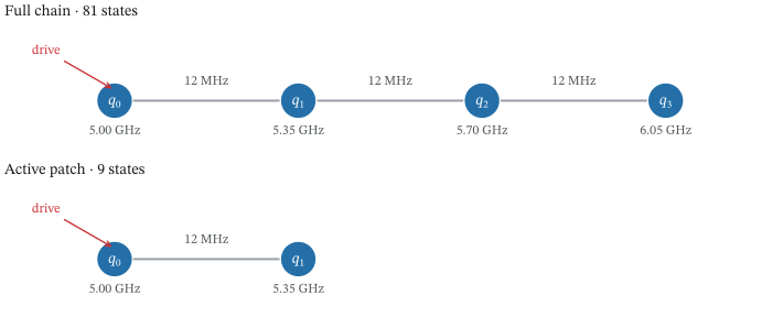
The reduced model has 9 basis states. The removed spectators contribute Hamiltonian corrections; labels show bare parameters. PDF
Simulate the same pulse in the reduced model
sequence.simulate() runs the full chip, and patch.simulate() runs the
schedule on the reduced chip. Compare the driven qubit’s excited-state
population.
times = np.linspace(0.0, 80.0, 321)

full_result = sequence.simulate(tlist=times)
reduced_result = patch.simulate(tlist=times)

full_population = np.asarray(full_result.population("q0", level=1)).real
reduced_population = np.asarray(reduced_result.population("q0", level=1)).real
population_residual = np.abs(full_population - reduced_population)
Plot the population and difference
figure, (population_axis, residual_axis) = plt.subplots(
    2,
    1,
    figsize=(7.2, 5.6),
    height_ratios=(3.0, 1.15),
    sharex=True,
    layout="constrained",
)

population_axis.plot(times, full_population, color="#16181C", linewidth=2.4, label="full chip (81 states)")
population_axis.plot(
    times,
    reduced_population,
    color="#C92F33",
    linewidth=1.6,
    linestyle="--",
    label="reduced model (9 states)",
)
population_axis.set_ylabel(r"$P(q_0=1)$")
population_axis.set_ylim(-0.02, 1.02)
population_axis.legend(loc="upper left")

display_residual = np.maximum(population_residual, 1.0e-10)
residual_axis.semilogy(times, display_residual, color="#C92F33", linewidth=1.8)
residual_axis.set(
    xlabel="Time (ns)",
    ylabel="Absolute residual",
    ylim=(1.0e-10, 2.0e-2),
)

figure_path = "../docs/images/reduce_and_replay.svg"

figure.savefig(figure_path)
plt.show()
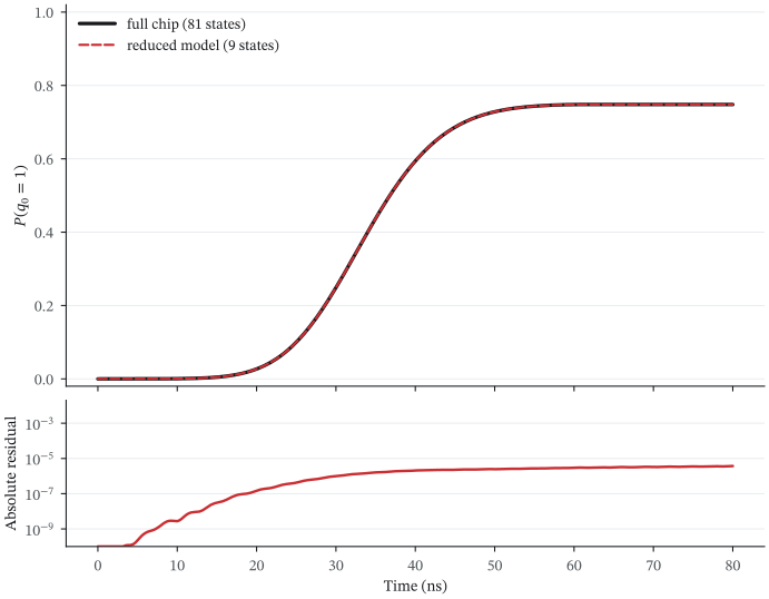
The full and reduced trajectories overlap; the lower panel resolves their absolute difference. Values below 10⁻¹⁰ are floored for display only. PDF
Inspect the elimination report
Each entry in patch.steps is an EliminationResult, whose describe()
report includes frequency shifts, inherited loss, coupling ratios, and
approximation notes. The kept Hamiltonian corrections set the reduced
dynamics, and the original device parameters do not change.
Show the built-in reports
for step in patch.steps:
    print(step.describe())
Output:
Elimination fold report (method='sw')
─────────────────────────────────────
q2: freq 5.7 → 5.69959 GHz   (Lamb shift -0.411 MHz)
validity: c23 g/Δ=0.034 ✓ (< 0.1) · min block gap 0.35 GHz
dropped: counter-rotating terms · ring-up transients · higher-order (>2) corrections
notes:
  - Retained the full second-order Hamiltonian correction and each transformed channel from the removed components; inherited decay remains collective and separate from intrinsic survivor noise.
Elimination fold report (method='sw')
─────────────────────────────────────
q1: freq 5.35 → 5.34959 GHz   (Lamb shift -0.412 MHz)
validity: c12 g/Δ=0.034 ✓ (< 0.1) · min block gap 0.35 GHz
dropped: counter-rotating terms · ring-up transients · higher-order (>2) corrections
notes:
  - Retained the full second-order Hamiltonian correction and each transformed channel from the removed components; inherited decay remains collective and separate from intrinsic survivor noise.
To remove a specific device directly, use
eliminate(chip, "q3", method="sw"), then inspect the returned .chip and
.describe(). method="exact" uses the kept block of the diagonalized model
instead of the second-order Schrieffer–Wolff approximation. Both methods use
the declared finite Hilbert space. Eliminating a coupling keeps both
endpoints.
Check the reduction error
A small coupling-to-detuning ratio is a diagnostic, not a guarantee of accurate
dynamics. Here we also check the full/reduced population difference against
5(g/Δ)², with the retained–eliminated boundary. The factor of five allows for
multilevel and finite-pulse effects. When you change the experiment, increase
hops to keep more neighbours and compare again.
Numerical checks and record
import json

full_dimension = int(np.prod(chip.dims))
reduced_dimension = int(np.prod(patch.chip.dims))
same_schedule = sequence.settings["entries"] == patch.sequence.settings["entries"]

validity_records = [
    record
    for eliminated_device in patch.validity.values()
    for record in eliminated_device.values()
]
max_g_over_delta = max(float(record["g_over_delta"]) for record in validity_records)
minimum_block_gap = min(float(record["min_block_gap"]) for record in validity_records)
all_folds_valid = all(bool(record["is_valid"]) for record in validity_records)

boundary_detuning = abs(float(chip.freq("q2")) - float(chip.freq("q1")))
boundary_ratio = coupling_strength / boundary_detuning
residual_tolerance = 5.0 * boundary_ratio**2
maximum_residual = float(np.max(population_residual))

if not all_folds_valid:
    raise RuntimeError("The active patch contains an invalid elimination step.")
if maximum_residual >= residual_tolerance:
    raise RuntimeError("The reduced dynamics exceed the validity-derived tolerance.")
if not same_schedule:
    raise RuntimeError("The reduced sequence does not preserve the scheduled entries.")
if tuple(device.label for device in chip.devices) != ("q0", "q1", "q2", "q3"):
    raise RuntimeError("active_patch() mutated the original chip.")

reduction_receipt = {
    "active_labels": list(patch.active_labels),
    "all_folds_valid": all_folds_valid,
    "eliminated_labels": list(patch.eliminated_labels),
    "figure": figure_path,
    "full_dimension": full_dimension,
    "maximum_population_residual": maximum_residual,
    "maximum_g_over_delta": max_g_over_delta,
    "minimum_block_gap_ghz": minimum_block_gap,
    "original_chip_unchanged": tuple(device.label for device in chip.devices) == ("q0", "q1", "q2", "q3"),
    "peak_full_population": float(np.max(full_population)),
    "reduced_dimension": reduced_dimension,
    "reduction_method": "sw",
    "residual_tolerance": residual_tolerance,
    "same_schedule": same_schedule,
}

print(f"RESULT reduction={json.dumps(reduction_receipt, sort_keys=True, separators=(',', ':'))}")
Output:
RESULT reduction={"active_labels":["q0","q1"],"all_folds_valid":true,"eliminated_labels":["q3","q2"],"figure":"../docs/images/reduce_and_replay.svg","full_dimension":81,"maximum_g_over_delta":0.03432606492529982,"maximum_population_residual":3.71427726397755e-06,"minimum_block_gap_ghz":0.3495885714285709,"original_chip_unchanged":true,"peak_full_population":0.7480171143273048,"reduced_dimension":9,"reduction_method":"sw","residual_tolerance":0.0058775348055535755,"same_schedule":true}
Other changes to the model
Use with_params() to change numerical parameters, as the spectrum
guide does during a sweep. chip.partition()
separates independent components exactly, but an active patch approximates
coupled spectators. If shared Hamiltonian terms, loss, or drive crosstalk keep
components in a joint solve, inspect partition.notes.
A default port on an eliminated linear resonator can follow the reduction into one unprojected Fock-space survivor. The transformed operator keeps its Purcell loss and output coupling. Unsupported port reductions raise. Coherent inputs and output-field observables still need the complete network solve.