Purcell filtering and T1

Compare two circuits: how much does a Purcell filter improve T1, and does it preserve the readout bandwidth? Include intrinsic loss in every mode. The readout guide covers the fridge wiring and measured S parameters. Frequencies are in GHz and times in ns.

Declare the two circuits

Both circuits use the same bare qubit and readout parameters:

Element	Frequency	Intrinsic loss	Coupling
Transmon	5 GHz	T1 = 60 µs	g = 105 MHz to readout
Readout resonator	7 GHz	Q = 200,000	Unfiltered external linewidth = 1 MHz
Filter resonator, when present	7.02 GHz	Q = 100,000	External linewidth = 230 MHz

The unfiltered circuit is qubit–readout–line. In the filtered circuit, a 7.02 GHz resonator sits between the readout and the line. Its coupling J is chosen to retain approximately 1 MHz of external readout linewidth:

\[\kappa_{\rm eff}(\omega)\simeq \frac{(2\pi J)^2\kappa_f}{(\kappa_f/2)^2+(\omega-\omega_f)^2}.\]

This broad-filter estimate suppresses escape near the qubit while keeping readout escape fast. The simulation also includes filter intrinsic loss. See Sete et al..

import numpy as np
from quchip import (
    Capacitive, Chip, DuffingTransmon, PortNetwork, QuantumSequence,
    Resonator, RWA,
)


q = DuffingTransmon(
    freq=5.0, anharmonicity=-0.2, levels=3, T1=60_000.0, label="q",
)
r = Resonator(freq=7.0, levels=2, internal_quality_factor=200_000, label="r")
qr = Capacitive(q, r, g=0.105, label="qr")
kappa_ext = 2 * np.pi * 0.001

line = PortNetwork(label="feedline")
line.expose("feedline", at=line.port("feed", target=r, rate=kappa_ext))
unfiltered = Chip([q, r], [qr], port_network=line, frame="lab", approximation=RWA())

Keep the same qubit, readout, and coupling. Add the filter and move the line’s coupling port from the readout to the filter:

f = Resonator(freq=7.02, levels=2, internal_quality_factor=100_000, label="f")
kappa_f = 2 * np.pi * 0.230
detuning = 2 * np.pi * (f.freq - r.freq)
J = np.sqrt(kappa_ext * kappa_f * (1 + (2 * detuning / kappa_f)**2)) / (4 * np.pi)
rf = Capacitive(r, f, g=J, label="rf")

filtered_line = PortNetwork(label="feedline")
filtered_line.expose("feedline", at=filtered_line.port("feed", target=f, rate=kappa_f))
filtered = Chip(
    [q, r, f], [qr, rf], port_network=filtered_line, frame="lab", approximation=RWA(),
)
chips = {"Unfiltered": unfiltered, "Filtered": filtered}

Draw the two circuit configurations

import shutil
import matplotlib.pyplot as plt

plt.style.use("../_static/quchip.mplstyle")
plt.rcParams["text.usetex"] = bool(shutil.which("latex"))
ink, muted = "#16181C", "#50565A"
fig, axes = plt.subplots(2, 1, figsize=(7.2, 5.8), layout="constrained")
for axis, filtered_circuit in zip(axes, [False, True]):
    axis.set(xlim=(-0.1, 11.3), ylim=(-1.0, 3.5), aspect="equal")
    axis.axis("off")
    axis.text(0, 3.15, "(b) With Purcell filter" if filtered_circuit else "(a) Without filter",
              fontsize=11, color=ink)
    modes = [(1.0, "Transmon", "junction"), (4.2, "Readout", "inductor")]
    if filtered_circuit:
        modes.append((7.4, "Purcell filter", "inductor"))
    for x, name, kind in modes:
        axis.text(x, 2.55, name, ha="center", color=muted, fontsize=10.5)
        # Each mode has a shunt capacitor and a Josephson junction or inductor.
        left, right = x - 0.45, x + 0.45
        axis.plot([left, right], [2, 2], color=ink, lw=1.5)
        axis.plot([left, right], [0.3, 0.3], color=ink, lw=1.5)
        axis.plot([left, left], [2, 1.25], color=ink, lw=1.5)
        axis.plot([left, left], [1.05, 0.3], color=ink, lw=1.5)
        axis.hlines([1.05, 1.25], left - 0.22, left + 0.22, color=ink, lw=1.5)
        axis.plot([right, right], [2, 1.5], color=ink, lw=1.5)
        axis.plot([right, right], [0.8, 0.3], color=ink, lw=1.5)
        if kind == "junction":
            axis.plot([right, right], [1.5, 0.8], color=ink, lw=1.5)
            axis.plot([right - 0.17, right + 0.17], [1.35, 0.95], color=ink, lw=1.5)
            axis.plot([right - 0.17, right + 0.17], [0.95, 1.35], color=ink, lw=1.5)
        else:
            phase = np.linspace(0, 8 * np.pi, 161)
            axis.plot(right + 0.16 * np.sin(phase), 1.5 - 0.7 * phase / (8 * np.pi), color=ink, lw=1.5)
        axis.plot([x, x], [0.3, 0.1], color=ink, lw=1.5)
        for y, width in [(0.1, 0.32), (-0.02, 0.21), (-0.14, 0.1)]:
            axis.plot([x - width, x + width], [y, y], color=ink, lw=1.3)
        parameters = {"Transmon": r"5 GHz" + "\n" + r"Intrinsic $T_1$ = 60 $\mu$s",
                      "Readout": r"7 GHz" + "\n" + r"$Q_i$ = 200,000",
                      "Purcell filter": r"7.02 GHz" + "\n" + r"$Q_i$ = 100,000"}
        axis.text(x, -0.42, parameters[name], ha="center", va="top", fontsize=9.5, color=muted)
    # Capacitive connections: g, then J when present, then coupling to the line.
    connections = [(1.45, 3.75, r"$g$ = 105 MHz")]
    if filtered_circuit:
        connections.append((4.65, 6.95, rf"$J$ = {1000 * J:.2f} MHz"))
    connections.append((7.85 if filtered_circuit else 4.65, 10.35, ""))
    for start, end, label in connections:
        center = (start + end) / 2
        axis.plot([start, center - 0.10], [2, 2], color=ink, lw=1.5)
        axis.plot([center + 0.10, end], [2, 2], color=ink, lw=1.5)
        axis.vlines([center - 0.10, center + 0.10], 1.73, 2.27, color=ink, lw=1.5)
        if label:
            axis.text(center, 1.52, label, ha="center", va="top", fontsize=9.5, color=muted)
    axis.text(10.35, 2.55, "Feedline", ha="center", fontsize=10.5, color=muted)
    axis.plot([10.35, 10.35], [2, 1.55], color=ink, lw=1.5)
    axis.plot([10.35, 10.18, 10.52, 10.18, 10.52, 10.35],
              [1.55, 1.4, 1.15, 0.9, 0.65, 0.5], color=ink, lw=1.5)
    axis.plot([10.35, 10.35], [0.5, 0.1], color=ink, lw=1.5)
    axis.text(10.67, 1.05, r"$Z_0$", va="center", fontsize=10.5, color=ink)
    for y, width in [(0.1, 0.32), (-0.02, 0.21), (-0.14, 0.1)]:
        axis.plot([10.35 - width, 10.35 + width], [y, y], color=ink, lw=1.3)
    linewidth = r"$\kappa_f/2\pi$ = 230 MHz" if filtered_circuit else r"$\kappa_{\mathrm{ext}}/2\pi$ = 1 MHz"
    axis.text(10.6, -0.42, linewidth, ha="right", va="top", fontsize=9.5, color=muted)
fig.savefig("slh_circuits.svg")
plt.close(fig)

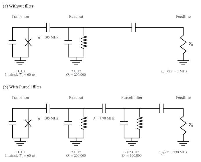
The filter moves the feedline coupling from the readout to a second resonator. J is chosen to preserve the readout bandwidth. Intrinsic losses are specified by T₁ and Qᵢ; Z₀ represents the matched feedline bath. PDF

Prepare one excitation and let it decay

Prepare the qubit-like eigenstate of the resolved RWA model. Each circuit uses the same time grid and records all local occupations.

times = np.r_[np.linspace(0, 100, 201), np.linspace(100, 120_000, 1201)[1:]]
results = {}
occupations = {}
for name, chip in chips.items():
    dressed = chip.resolve().dress(overlap_threshold=0.0)
    label = (1,) + (0,) * (len(chip.devices) - 1)
    assert dressed.assignment_overlaps[label] > 0.99
    initial = dressed.eigenstates[dressed.state_map[label]]
    nops = chip.e_ops(**{device.label: "n" for device in chip.devices})
    result = QuantumSequence(chip).simulate(
        tlist=times, initial_state=initial, e_ops=nops, check_truncation=False,
    )
    results[name] = result
    occupations[name] = np.array([np.real(result.expect(key)) for key in nops])

Fit the exponential tail of the qubit occupation to extract T1.

lifetimes = {}
for name, occupation in occupations.items():
    fit = (times >= 1000) & (occupation[0] > 1e-3)
    slope, intercept = np.polyfit(times[fit], np.log(occupation[0, fit]), 1)
    np.testing.assert_allclose(occupation[0, fit], np.exp(intercept + slope * times[fit]), rtol=1e-3)
    lifetimes[name] = -1 / slope

Plot qubit decay

fig, axis = plt.subplots(figsize=(6.6, 3.7), layout="constrained")
for (name, occupation), color in zip(occupations.items(), ["#C92F33", "#246FA8"]):
    axis.plot(times / 1000, occupation[0], color=color, lw=2.2,
              label=rf"{name}: {lifetimes[name] / 1000:.1f} $\mu$s")
axis.plot(times / 1000, np.exp(-times / 60_000), color="#16181C", ls=":", lw=1.8,
          label=r"Intrinsic qubit: 60 $\mu$s")
axis.set(xlabel=r"Time ($\mu$s)", ylabel="Qubit occupation", xlim=(0, 120), ylim=(0, 1.02))
axis.legend()
fig.savefig("slh_t1_budget.svg")
plt.close(fig)

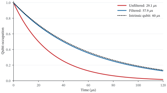
The filter raises T1 from 29.1 to 57.9 µs, approaching the qubit’s intrinsic 60 µs limit. PDF

Where the excitation is lost

The integrated loss budget explains the T1 improvement:

Bath	Without filter	With filter
Qubit intrinsic	48.3%	96.2%
Readout intrinsic	1.75%	3.48%
Filter intrinsic	—	<0.001%
Feedline	49.9%	0.329%

These are fractions of the excitation lost by 120 µs; excitation still in the circuit is excluded. Filtering suppresses feedline loss, leaving the intrinsic qubit and readout losses as the limit.

Integrate the losses and check excitation balance

lost = {}
for name, result in results.items():
    lost[name] = {key: np.asarray(result.collapse_integral(key)) for key in result.collapse_channels}
    np.testing.assert_allclose(occupations[name].sum(axis=0) + sum(lost[name].values()), 1, atol=1e-5, rtol=0)

The balance applies to this vacuum, single-excitation decay model.

Verify the lifetime and bandwidth

Grid and local-level refinement change T1 and integrated channel losses by less than 1e-4. The unfiltered T1 also agrees with the dispersive estimate.

Check the decay estimate, sampling, and local levels

kappa_int = 2 * np.pi * r.freq / r.internal_quality_factor
mixing = (unfiltered.coupling("qr").g / (q.freq - r.freq))**2
estimate = 1 / (1 / q.T1 + (kappa_int + 2 * np.pi * 0.001) * mixing)
np.testing.assert_allclose(lifetimes["Unfiltered"], estimate, rtol=0.02)

r3 = Resonator(freq=r.freq, levels=3, internal_quality_factor=r.internal_quality_factor, label="r")
f3 = Resonator(freq=f.freq, levels=3, internal_quality_factor=f.internal_quality_factor, label="f")
line3 = PortNetwork(label="feedline")
line3.expose("feedline", at=line3.port("feed", target=f3, rate=kappa_f))
expanded = Chip(
    [q, r3, f3],
    [Capacitive(q, r3, g=qr.g, label="qr"), Capacitive(r3, f3, g=J, label="rf")],
    port_network=line3, frame="lab", approximation=RWA(),
)
fine_grid = np.sort(np.r_[times, (times[:-1] + times[1:]) / 2])
for checked_chip, grid in ((filtered, fine_grid), (expanded, times)):
    dressed = checked_chip.resolve().dress(overlap_threshold=0.0)
    initial = dressed.eigenstates[dressed.state_map[(1, 0, 0)]]
    nops = checked_chip.e_ops(q="n")
    checked = QuantumSequence(checked_chip).simulate(
        tlist=grid, initial_state=initial, e_ops=nops, check_truncation=False,
    )
    nq = np.real(checked.expect(next(iter(nops))))
    tail = (grid >= 1000) & (nq > 1e-3)
    checked_t1 = -1 / np.polyfit(grid[tail], np.log(nq[tail]), 1)[0]
    np.testing.assert_allclose(checked_t1, lifetimes["Filtered"], rtol=1e-4)
    for key in lost["Filtered"]:
        np.testing.assert_allclose(checked.collapse_integral(key)[-1], lost["Filtered"][key][-1], rtol=1e-4)

Start with one bare readout photon and fit the ring-down after the fast filter transient. This measures the total loaded linewidth, including intrinsic loss.

ring_times = np.linspace(0, 1500, 751)
linewidths = []
for name, chip in chips.items():
    nops = chip.e_ops(r="n")
    ring = QuantumSequence(chip).simulate(
        tlist=ring_times, initial_state=chip.bare_state(r=1),
        e_ops=nops, check_truncation=False,
    )
    nr = np.real(ring.expect(next(iter(nops))))
    fit = (ring_times >= 100) & (ring_times <= 600)
    kappa = -np.polyfit(ring_times[fit], np.log(nr[fit]), 1)[0]
    linewidths.append(kappa / (2 * np.pi) * 1000)
np.testing.assert_allclose(linewidths[1], linewidths[0], rtol=0.05)

The loaded linewidth is 1.033 MHz without the filter and 1.051 MHz with it, within the 5% design tolerance of the broad-filter estimate. A network.filter() applies a transfer function to the signal path. It cannot provide this T1 protection; that requires a coupled resonator in the quantum model, which changes the decay channels.